SKEDSOFT

To keep things simple, we start with the case of a passive learning agent using a state-based representation in a fully observable environment. In passive learning, the agent's policy 1r is fixed: in state 8, it always executes the action 1r(8) . Its goal is simply to learn how good the policy is-that is, to learn the utility function U'��" ( 8 ). We will use as our example the 4 x 3 world introduced in Chapter 17. Figure 21.1 shows a policy for that world and the corresponding utilities. Clearly, the passive learning task is similar to the policy evaluation task, part of the poli cy iteration algorithm described in Section 17.3. The main difference is that the passive learning agent does not know the transition model P(8' 1 8, a), which specifies the probability of reaching state 81 from state 8 after doing action a; nor does it know the reward function R( 8 ), which specifies the reward for each state.

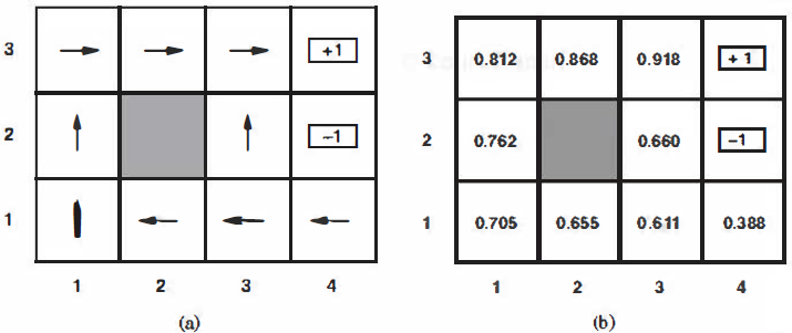
Figure 21.1 (a) A policy 1r for the 4 X 3 world; this policy happens to be optimal with rewards of R( s) = - 0.04 in the nonterminal states and no discounting. (b) The utilities of the states in the 4 X 3 world, given policy 1r

The agent executes a set of trials in the environment using its policy 1r. In each trial, the agent starts in state (1, 1) and experiences a sequence of state transitions until it reaches one of the terminal states, (4,2) or (4,3). Its percepts supply both the current state and the reward received in that state. Typical trials might look like this:

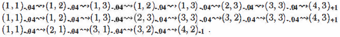
Note that each state percept is subscripted with the reward received. The object is to use the information about rewards to leam the expected utility U'��" ( 8) associated with each nonterm ina] state 8. The utility is defined to be the expected sum of (discounted) rewards obtained if

policy 1r is followed. As in Equation (17.2) on page 650, we write

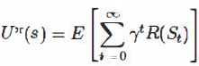
where R(s) is the reward for a state, St (a random variable) is the state reached at time t when executing policy 1r, and So= s. We will include a discount factor 1 in all of our equations, but for the 4 x 3 world we will set 1 = 1.

Direct utility estimation: A simple method for direct utility estimation was invented in the late 1950s in the area of adaptive control theory by Widrow and Hoff (1960). The idea is that the utility of a state is the expected total reward from that state onward (called the expected reward-to-go), and each trial provides a sample of this quantity for each state visited. For example, the first trial in the set of three given earlier provides a sample total reward of 0. 72 for state (1, 1 ), two samples of 0.76 and 0.84 for (1,2), two samples of 0.80 and 0.88 for (1,3), and so on. Thus, at the end of each sequence, the algorithm calculates the observed reward-to-go for each state and updates the estimated utility for that state accordingly, just by keeping a running average for each state in a table. In the limit of infinitely many trials, the sample average will converge to the true expectation in Equation (21.1 ).

It is clear that direct utility estimation is just an instance of supervised learning where each example has the state as input and the observed reward-to-go as output. This means that we have reduced reinforcement learning to a standard inductive learning problem, as discussed in Chapter 18. Section 21.4 discusses the use of more powerful kinds of representations for the utility function. Learning techniques for those representations can be applied directly to the observed data.

Direct utility estimation succeeds in reducing the reinforcement learning problem to an inductive learning problem, about which much is known. Unfortunately, it misses a very important source of information, namely, the fact that the utilities of states are not independent! The utility of each state equals its own reward plus the expected utility of its successor states. That is, the utility values obey the Bellman equations for a fixed policy (see also Equation (17. 10)):

By ignoring the connections between states, direct utility estimation misses opportunities for leaming. For example, the second of the three trials given earlier reaches the state (3,2), which has not previously been visited. The next transition reaches (3,3), which is known from the first trial to have a high utility. The Bellman equation suggests immediately that (3,2) is also likely to have a high utility, because it leads to (3,3), but direct utility estimation learns nothing until the end of the trial More broadly, we can view direct utility estimation as searching for U in a hypothesis space that is much larger than it needs to be, in that it includes many functions that violate the Bellman equations. For this reason, the algorithm often converges very slowly.