SKEDSOFT
Properties of Depth First Search: Let us now examine some properties of the DFS algorithm. The algorithm takes exponential time. If N is the maximum depth of a node in the search space, in the worst case the algorithm will take time O(bd). However the space taken is linear in the depth of the search tree, O(bN). Note that the time taken by the algorithm is related to the maximum depth of the search tree. If the search tree has infinite depth, the algorithm may not terminate. This can happen if the search space is infinite. It can also happen if the search space contains cycles. The latter case can be handled by checking for cycles in the algorithm. Thus Depth First Search is not complete.
Depth Limited Search: A variation of Depth First Search circumvents the above problem by keeping a depth bound. Nodes are only expanded if they have depth less than the bound. This algorithm is known as depth-limited search.
- Depth limited search (limit)
- Let fringe be a list containing the initial state
- Loop if fringe is empty return failure Node <- remove-first (fringe)
- if Node is a goal
- then return the path from initial state to Node
- else if depth of Node = limit return cutoff
- else add generated nodes to the front of fringe
- End Loop
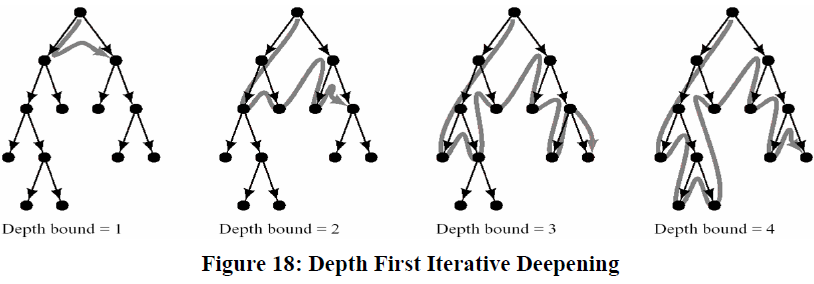
Depth-First Iterative Deepening (DFID): First do DFS to depth 0 (i.e., treat start node as having no successors), then, if no solution found, do DFS to depth 1, etc.
- DFID
- until solution found do
- DFS with depth cutoff c
- c = c 1
Advantage
• Linear memory requirements of depth-first search
• Guarantee for goal node of minimal depth
Procedure: Successive depth-first searches are conducted – each with depth bounds increasing by 1
Properties: For large d the ratio of the number of nodes expanded by DFID compared to that of DFS is given by b/(b-1). For a branching factor of 10 and deep goals, 11% more nodes expansion in iterative-deepening search than breadth-first search The algorithm is
- Complete
- Optimal/Admissible if all operators have the same cost. Otherwise, not optimal but guarantees finding solution of shortest length (like BFS).
- Time complexity is a little worse than BFS or DFS because nodes near the top of the search tree are generated multiple times, but because almost all of the nodes are near the bottom of a tree, the worst case time complexity is still exponential, O(bd) If branching factor is b and solution is at depth d, then nodes at depth d are generated once, nodes at depth d-1 are generated twice, etc. Hence bd 2b(d-1) ... db <= bd / (1 - 1/b)2 = O(bd).
- Linear space complexity, O(bd), like DFS
Depth First Iterative Deepening combines the advantage of BFS (i.e., completeness) with the advantages of DFS (i.e., limited space and finds longer paths more quickly) This algorithm is generally preferred for large state spaces where the solution depth is unknown. There is a related technique called iterative broadening is useful when there are many goal nodes. This algorithm works by first constructing a search tree by expanding only one child per node. In the 2nd iteration, two children are expanded, and in the ith iteration I children are expanded.