SKEDSOFT

Review of Probability Theory: The primitives in probabilistic reasoning are random variables. Just like primitives in Propositional Logic are propositions. A random variable is not in fact a variable, but a function from a sample space S to another space, often the real numbers.

For example, let the random variable Sum (representing outcome of two die throws) be defined thus:
Sum(die1, die2) = die1 die2

Each random variable has an associated probability distribution determined by the underlying distribution on the sample space
Continuing our example : P(Sum = 2) = 1/36,
P(Sum = 3) = 2/36, . . . , P(Sum = 12) = 1/36

Consdier the probabilistic model of the fictitious medical expert system mentioned before. The sample space is described by 8 binary valued variables.

Visit to Asia? A
Tuberculosis? T
Either tub. or lung cancer? E
Lung cancer? L
Smoking? S
Bronchitis? B
Dyspnoea? D
Positive X-ray? X

There are 28 = 256 events in the sample space. Each event is determined by a joint instantiation of all of the variables.

S = {(A = f, T = f,E = f,L = f, S = f,B = f,D = f,X = f),
(A = f, T = f,E = f,L = f, S = f,B = f,D = f,X = t), . . .
(A = t, T = t,E = t,L = t, S = t,B = t,D = t,X = t)}

Since S is defined in terms of joint instantations, any distribution defined on it is called a joint distribution. ll underlying distributions will be joint distributions in this module. The variables {A,T,E, L,S,B,D,X} are in fact random variables, which ‘project’ values.

L(A = f, T = f,E = f,L = f, S = f,B = f,D = f,X = f) = f
L(A = f, T = f,E = f,L = f, S = f,B = f,D = f,X = t) = f
L(A = t, T = t,E = t,L = t, S = t,B = t,D = t,X = t) = t

Each of the random variables {A,T,E,L,S,B,D,X} has its own distribution, determined by the underlying joint distribution. This is known as the margin distribution. For example, the distribution for L is denoted P(L), and this distribution is defined by the two probabilities P(L = f) and P(L = t). For example,

P(L = f)
= P(A = f, T = f,E = f,L = f, S = f,B = f,D = f,X = f)
P(A = f, T = f,E = f,L = f, S = f,B = f,D = f,X = t)
P(A = f, T = f,E = f,L = f, S = f,B = f,D = t,X = f)
. . .
P(A = t, T = t,E = t,L = f, S = t,B = t,D = t,X = t)
P(L) is an example of a marginal distribution.

Here’s a joint distribution over two binary value variables A and B

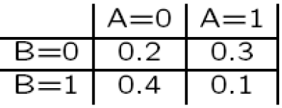
We get the marginal distribution over B by simply adding up the different possible values of A for any value of B (and put the result in the “margin”).

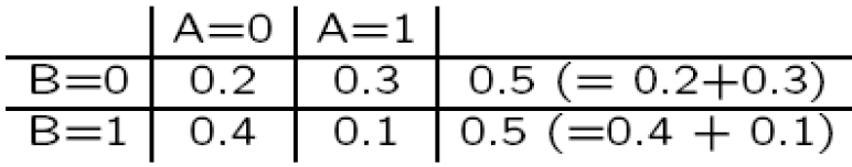
In general, given a joint distribution over a set of variables, we can get the marginal distribution over a subset by simply summing out those variables not in the subset.

In the medical expert system case, we can get the marginal distribution over, say, A,D by simply summing out the other variables:

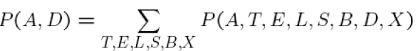
However, computing marginals is not an easy task always. For example,
P(A = t,D = f)
= P(A = t, T = f,E = f,L = f, S = f,B = f,D = f,X = f)
P(A = t, T = f,E = f,L = f, S = f,B = f,D = f,X = t)
P(A = t, T = f,E = f,L = f, S = f,B = t,D = f,X = f)
P(A = t, T = f,E = f,L = f, S = f,B = t,D = f,X = t)
. . .
P(A = t, T = t,E = t,L = t, S = t,B = t,D = f,X = t)