SKEDSOFT
Concept of stability:
When considering the design and analysis of feedback control systems, stability is of the utmost importance. From a practical point of view, a closed-loop feedback system that is unstable is of little value. As with all such general statements, there are exceptions; but for our purposes, we will declare that all our control designs must result in a closed-loop stable system. Many physical systems are inherently open-loop unstable, and some systems are even designed to be open-loop unstable. Most modern fighter aircraft are open-loop unstable by design, and without active feedback control assisting the pilot, they cannot fly. Active control is introduced by engineers to stabilize the unstable system—that is, the aircraft—so that other considerations, such as transient performance, can be addressed. Using feedback, we can stabilize unstable systems and then with a judicious selection of controller parameters, we can adjust the transient performance. For open-loop stable systems, we still use feedback to adjust the closed-loop performance to meet the design specifications.
These specifications take the form of steady-state tracking errors, percent overshoot, settling time, time to peak, and the other. We can say that a closed-loop feedback system is either stable or it is not stable. This type of stable/not stable characterization is referred to as absolute stability. A system possessing absolute stability is called a stable system—the label of absolute is dropped. Given that a closed-loop system is stable, we can further characterize the degree of stability. This is referred to as relative stability. The pioneers of aircraft design were familiar with the notion of relative stability—the more stable an aircraft was, the more difficult it was to maneuver (that is, to turn). One outcome of the relative instability of modern fighter aircraft is high maneuverability. A fighter aircraft is less stable than a commercial transport, hence it can maneuver more quickly. In fact, the motions of a fighter aircraft can be quite violent to the "passengers." We can determine that a system is stable (in the absolute sense) by determining that all transfer function poles lie in the left-half s-plane, or equivalently, that all the eigenvalues of the system matrix A lie in the left-half s-plane. Given that all the poles (or eigenvalues) are in the left-half s-plane, we investigate relative-stability by examining the relative locations of the poles (or eigenvalues). A stable system is defined as a system with a bounded (limited) system response. That is, if the system is subjected to a bounded input or disturbance and the response is bounded in magnitude, the system is said to be stable. A stable system is a dynamic system with a bounded response to a bounded input.
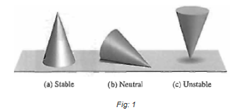
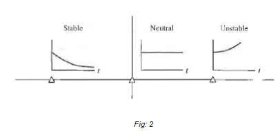
The concept of stability can be illustrated by considering a right circular cone placed on a plane horizontal surface. If the cone is resting on its base and is tipped slightly, it returns to its original equilibrium position. This position and response are said to be stable. If the cone rests on its side and is displaced slightly, it rolls with no tendency to leave the position on its side. This position is designated as the neutral stability. On the other hand, if the cone is placed on its tip and released, it falls onto its side. This position is said to be unstable. These three positions are illustrated in Figure 1. The stability of a dynamic system is defined in a similar manner. The response to a displacement, or initial condition, will result in either a decreasing, neutral, or increasing response. Specifically, it follows from the definition of stability that a linear system is stable if and only if the absolute value of its impulse response g(t), integrated over an infinite range, is finite The location in the s-plane of the poles of a system indicates the resulting transient response. The poles in the left-hand portion of the s-plane result in a decreasing response for disturbance inputs. Similarly, poles on the jω-axis and in the right-hand plane result in a neutral and an increasing response, respectively, for a disturbance input. This division of the s-plane is shown in Figure 2.
Clearly, the poles of desirable dynamic systems must lie in the left-hand portion of the s-plane. In terms of linear systems, we recognize that the stability requirement may be defined in terms of the location of the poles of the closed-loop transfer function. The closed-loop system transfer function is written as
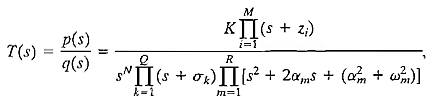
where q(s) = Δ(s) = 0 is the characteristic equation whose roots are the poles of the closed-loop system. The output response for an impulse function input (when N = 0) is then
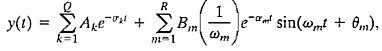
where Ak and Bm are constants that depend on σk, Zi, αm, K, and ωm. To obtain a bounded response, the poles of the closed-loop system must be in the left-hand portion of the s-plane. Thus, a necessary and sufficient condition for a feedback system to be stable is that all the poles of the system transfer function have negative real parts. A system is stable if all the poles of the transfer function are in the left-hand s-plane. A system is not stable if not all the roots are in the left-hand plane. If the characteristic equation has simple roots on the imaginary axis (jω-axis) with all other roots in the left half-plane, the steady-state output will be sustained oscillations for a bounded input, unless the input is a sinusoid (which is bounded) whose frequency is equal to the magnitude of the jω-axis roots. For this case, the output becomes unbounded. Such a system is called marginally stable, since only certain bounded inputs (sinusoids of the frequency of the poles) will cause the output to become unbounded. For an unstable system, the characteristic equation has at least one root in the right half of the s-plane or repeated jω roots; for this case, the output will become unbounded for any input.
