SKEDSOFT
General procedure for plotting Bode diagrams
First rewrite the sinusoidal transfer function G(jω)H(jω) as a product of basic factors. Then identify the corner frequencies associated with these basic factors. Finally, draw the asymptotic log-magnitude curves with proper slopes between the corner frequencies. The exact curve, which lies close to the asymptotic curve, can be obtained by adding proper corrections.
The phase-angle curve of G(jω)H(jω) can be drawn by adding the phase-angle curves of individual factors. The use of Bode diagrams employing asymptotic approximations requires much less time than other methods that may be used for computing the frequency response of a transfer function. The ease of plotting the frequency-response curves for a given transfer function and the ease of modification of the frequency-response curve as compensation is added are the main reasons why Bode diagrams are very frequently used in practice.
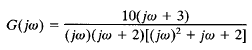
EXAMPLE: Draw the Bode diagram for the following transfer function:
Make corrections so that the log-magnitude curve is accurate. To avoid any possible mistakes in drawing the log-magnitude curve, it is desirable to put G(jω) in the following normalized form, where the low-frequency asymptotes for the first-order factors and the second-order factor are the O-dB line.
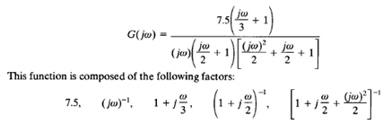
The corner frequencies of the third, fourth, and fifth terms are ω = 3, ω = 2, and ω = √2, respectively.
Note that the last term has the damping ratio of 0.3536.
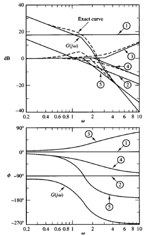
To plot the Bode diagram, the separate asymptotic curves for each of the factors are shown in Figure. The composite curve is then obtained by adding algebraically the individual curves, also shown in Figure.
Note that when the individual asymptotic curves are added at each frequency the slope of the composite curve is cumulative. Below ω = 0, the plot has the slope of -20 dB/decade. At the first corner frequency ω = 0, the slope changes to -60 dB/decade and continues to the next corner frequency ω= 2, where the slope becomes -80 dB/decade. At the last corner frequency ω = 3, the slope changes to -60 dB/decade.
Once such an approximate log-magnitude curve has been drawn, the actual curve can be obtained by adding corrections at each corner frequency and at frequencies one octave below and above the corner frequencies. For first-order factors (1 jωT)∓1, the corrections are ±3 dB at the corner frequency and ±1 dB at the frequencies one octave below and above the corner frequency.
Corrections necessary for the quadratic factor are done. The exact log magnitude curve for C(jω) is shown by a dashed curve in Figure. Note that any change in the slope of the magnitude curve is made only at the corner frequencies of the transfer function C(jω). Therefore, instead of drawing individual magnitude curves and adding them up, as shown, we may sketch the magnitude curve without sketching individual curves.
We may start drawing the lowest-frequency portion of the straight line (that is, the straight line with the slope - 20 dB/decade for ω < 0). As the frequency is increased, we get the effect of the complex-conjugate poles (quadratic term) at the corner frequency ω = 0.The complex conjugate poles cause the slopes of the magnitude curve to change from -20 to -60 dB/decade. At the next corner frequency, ω = 2, the effect of the pole is to change the slope to -80 dB/decade. Finally, at the corner frequency w = 3, the effect of the zero is to change the slope from -80 to -60 dB/decade.
For plotting the complete phase-angle curve, the phase-angle curves for all factors have to be sketched. The algebraic sum of all phase-angle curves provides the complete phase-angle curve, as shown in Figure.
