SKEDSOFT
General shapes of polar plots
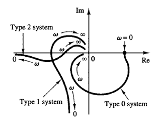
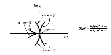
Fig: 1 Polar plots of type 0, type 1, and type 2 systems Fig: 2 Polar plots in the high-frequency range
The polar plots of a transfer function of the form
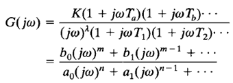
where n > m or the degree of the denominator polynomial is greater than that of the numerator, will have the following general shapes:
1. For λ = 0 or type 0 systems:
The starting point of the polar plot (which corresponds to ω = 0) is finite and is on the positive real axis. The tangent to the polar plot at ω = 0 is perpendicular to the real axis. The terminal point, which corresponds to ω = ∞, is at the origin, and the curve is tangent to one of the axes.
2. For λ = 1 or type 1 systems:
The jω term in the denominator contributes -900 to the total phase angle of G(jω) for 0 ≤ ω ≤ ∞. At ω = 0, the magnitude of G(jω) is infinity, and the phase angle becomes -900. At low frequencies, the polar plot is asymptotic to a line parallel to the negative imaginary axis. At ω = ∞, the magnitude becomes zero, and the curve converges to the origin and is tangent to one of the axes.
3. For λ = 2 or type 2 systems:
The (jω)2 term in the denominator contributes -1800 to the total phase angle of G(jω) for 0 ≤ W ≤ ∞. At ω = 0, the magnitude of G(jω) is infinity, and the phase angle is equal to -1800. At low frequencies, the polar plot is asymptotic to a line parallel to the negative real axis. At ω = ∞, the magnitude becomes zero, and the curve is tangent to one of the axes.
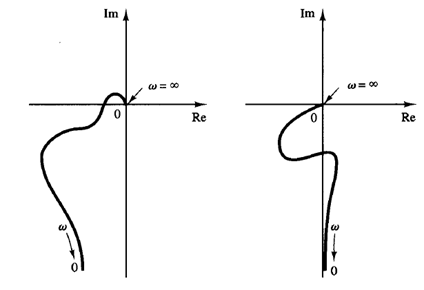
Fig: 3 Polar plots of transfer functions with numerator dynamics
The general shapes of the low-frequency portions of the polar plots of type 0, type 1, and type 2 systems are shown in Figure 1. It can be seen that, if the degree of the denominator polynomial of G(jω) is greater than that of the numerator, then the G(jω) loci converge to the origin clockwise. At ω = ∞, the loci are tangent to one or the other axes, as shown in Figure 2
