SKEDSOFT

Nyquist stability criterion

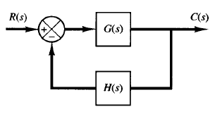
Fig: 1 closed loop system

Consider the closed-loop system shown in Figure 1. The closed-loop transfer function is

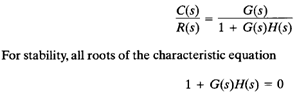
must lie in the left-half s plane. [It is noted that, although poles and zeros of the open loop transfer function G(s)H(s) may be in the right-half s plane, the system is stable if all the poles of the closed-loop transfer function (that is, the roots of the characteristic equation) are in the left-half s plane.]

The Nyquist stability criterion relates the open loop frequency response G(jω)H(jω) to the number of zeros and poles of 1 G(s)H(s) that lie in the right-half s plane. This criterion, derived by H. Nyquist, is useful in control engineering because the absolute stability of the closed-loop system can be determined graphically from open-loop frequency-response curves, and there is no need for actually determining the closed-loop poles.

 Analytically obtained open-loop frequency response curves, as well as those experimentally obtained, can be used for the stability analysis. This is convenient because, in designing a control system, it often happens that mathematical expressions for some of the components are not known; only their frequency-response data are available.

The Nyquist stability criterion is based on a theorem from the theory of complex variables. To understand the criterion, we shall first discuss mappings of contours in the complex plane.

We shall assume that the open-loop transfer function G(s)H(s) is representable as a ratio of polynomials in s. For a physically realizable system, the degree of the denominator polynomial of the closed-loop transfer function must be greater than or equal to that of the numerator polynomial. This means that the limit of G(s)H(s) as s approaches infinity is zero or a constant for any physically realizable system.