SKEDSOFT

Polar plot:

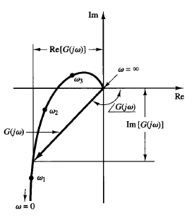
Fig: 1 Polar plot

The polar plot of a sinusoidal transfer function G(jω) is a plot of the magnitude of G(jω) versus the phase angle of G(jω) on polar coordinates as ω is varied from zero to infinity.

Thus, the polar plot is the locus of vectors as ω is varied from zero to infinity. Note that in polar plots a positive (negative) phase angle is measured counterclockwise (clockwise) from the positive real axis. The polar plot is often called the Nyquist plot. An example of such a plot is shown in Figure 1. Each point on the polar plot of G(jω) represents the terminal point of a vector at a particular value of ω. In the polar plot, it is important to show the frequency graduation of the locus. The projections of G(jω) on the real and imaginary axes are its real and imaginary components.

Both the magnitude and phase angle must be calculated directly for each frequency w in order to construct polar plots. Since the logarithmic plot is easy to construct, however, the data necessary for plotting the polar plot may be obtained directly from the logarithmic plot if the latter is drawn first and decibels are converted into ordinary magnitude. Or, of course, MATLAB may be used to obtain a polar plot G(jω) or to obtain and accurately for various values of ω in the frequency range of interest.

 An advantage in using a polar plot is that it depicts the frequency-response characteristics of a system over the entire frequency range in a single plot. One disadvantage is that the plot does not clearly indicate the contributions of each individual factor of the open-loop transfer function.

Integral and derivative factors

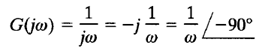
The polar plot of G (jω) = 1/ jωis the negative imaginary axis since

The polar plot of G(jω) = jω is the positive imaginary axis.