SKEDSOFT

Root-locus approach to control system design

In building a control system, we know that proper modification of the plant dynamics may be a simple way to meet the performance specifications. This, however, may not be possible in many practical situations because the plant may be fixed and may not be modified. Then we must adjust parameters other than those in the fixed plant. We assume that the plant is given and unalterable. The design problems, therefore, become those of improving system performance by insertion of a compensator. Compensation of a control system is reduced to the design of a filter whose characteristics tend to compensate for the undesirable and unalterable characteristics of the plant.

The root-locus method is a graphical method for determining the locations of all closed-loop poles from knowledge of the locations of the open-loop poles and zeros as some parameter (usually the gain) is varied from zero to infinity. The method yields a clear indication of the effects of parameter adjustment.

In practice, the root-locus plot of a system may indicate that the desired performance cannot be achieved just by the adjustment of gain. In fact, in some cases, the system may not be stable for all values of gain. Then it is necessary to reshape the root loci to meet the performance specifications. In designing a control system, if other than a gain adjustment is required, we must modify the original root loci by inserting a suitable compensator.

 Once the effects on the root locus of the addition of poles and/or zeros are fully understood, we can readily determine the locations of the pole(s) and zero(s) of the compensator that will reshape the root locus as desired. In essence, in the design by the root-locus method, the root loci of the system are reshaped through the use of a compensator so that a pair of dominant closed-loop poles can be placed at the desired location. (Often, the damping ratio and undamped natural frequency of a pair of dominant closed-loop poles are specified.)

Effects of the addition of poles:

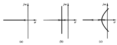
Fig 1: (a) Root-locus plot of a single-pole system; (b) root-locus plot of a two-pole system; (c) root-locus plot of a three-pole system

 The addition of a pole to the open-loop transfer function has the effect of pulling the root locus to the right, tending to lower the system's relative stability and to slow down the settling of the response. (Remember that the addition of integral control adds a pole at the origin, thus making the system less stable.) Figure 1 shows examples of root loci illustrating the effects of the addition of a pole to a single-pole system and the addition of two poles to a single pole system.

Effects of the addition of zeros:

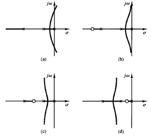
Fig 2: (a) Root-locus plot of a three-pole system; (b), (c), and (d) root-locus plots showing effects of addition of a zero to the three-pole system

 The addition of a zero to the open-loop transfer function has the effect of pulling the root locus to the left, tending to make the system more stable and to speed up the settling of the response. (Physically, the addition of a zero in the feed forward transfer function means the addition of derivative control to the system. The effect of such control is to introduce a degree of anticipation into the system and speed up the transient response.) Figure 2(a) shows the root loci for a system that is stable for small gain but unstable for large gain. Figures 2(b), (c), and (d) show root-locus plots for the system when a zero is added to the open-loop transfer function. Notice that when a zero is added to the system of Figure 2(a) it becomes stable for all values of gain.