SKEDSOFT

Transport lag of polar plot

The transport lag

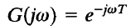
can be written

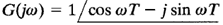
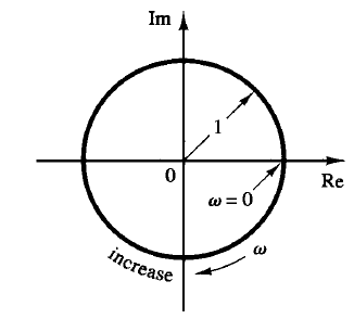
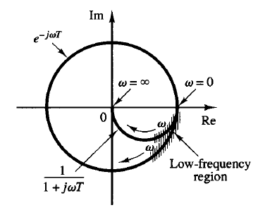
Fig: 1                                                                                                        Fig: 2

Since the magnitude of G(jω) is always unity and the phase angle varies linearly with ω, the polar plot of the transport lag is a unit circle, as shown in Figure1.

At low frequencies, the transport lag e^-jωT and the first-order lag 1/(1 jωT) behave similarly, as shown in Figure 2. The polar plots of e^-jωT and 1/(1 jωT) are tangent to each other at w = 0. This may be seen from the fact that, for ω << 1/T,

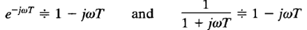
For ω >> 1/T, however, an essential difference exists between e^-jωT and 1/(1 jωT), as may also be seen from Figure 2