SKEDSOFT

Introduction: The naïve Bayesian classifier makes the assumption of class conditional independence, that is, given the class label of a tuple, the values of the attributes are assumed to be conditionally independent of one another. This simplifies computation. When the assumption holds true, then the naïve Bayesian classifier is the most accurate in comparison with all other classifiers. In practice, however, dependencies can exist between variables. Bayesian belief networks specify joint conditional probability distributions. They allow class conditional independencies to be defined between subsets of variables.

They provide a graphical model of causal relationships, on which learning can be performed. Trained Bayesian belief networks can be used for classification. Bayesian belief networks are also known as belief networks, Bayesian networks, and probabilistic networks. For brevity, we will refer to them as belief networks.

A belief network is defined by two components—a directed acyclic graph and a set of conditional probability tables (Figure 6.11). Each node in the directed acyclic graph represents a random variable. The variables may be discrete or continuous-valued. They may correspond to actual attributes given in the data or to “hidden variables” believed to form a relationship (e.g., in the case of medical data, a hidden variable may indicate a syndrome, representing a number of symptoms that, together, characterize a specific disease). Each arc represents a probabilistic dependence. If an arc is drawn from a node Y to a node Z, then Y is a parent or immediate predecessor of Z, and Z is a descendant of Y. Each variable is conditionally independent of its non-descendants in the graph, given its parents.

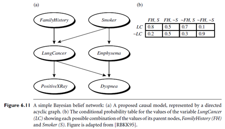Figure 6.11 is a simple belief network, adapted from [RBKK95] for six Boolean variables. The arcs in Figure 6.11(a) allow a representation of causal knowledge. For example, having lung cancer is influenced by a person’s family history of lung cancer, as well as whether or not the person is a smoker. Note that the variable Positive X-Ray is independent of whether the patient has a family history of lung cancer or is a smoker, given that we know the patient has lung cancer. In other words, once we know the outcome of the variable Lung Cancer, then the variables Family History and Smoker do not provide any additional information regarding Positive X Ray. The arcs also show that the variable Lung Cancer is conditionally independent of Emphysema, given its parents, Family History and Smoker.

A belief network has one conditional probability table (CPT) for each variable. The CPT for a variable Y specifies the conditional distribution P(Y|Parents(Y)), where Parents(Y) are the parents of Y. Figure 6.11(b) shows a CPT for the variable Lung Cancer. The conditional probability for each known value of Lung Cancer is given for each possible combination of values of its parents. For instance, from the upper leftmost and bottom rightmost entries, respectively, we see that

P(LungCancer = yes | FamilyHistory = yes, Smoker = yes) = 0.8

P(LungCancer = no | FamilyHistory = no, Smoker = no) = 0.9

Let X = (x1, : : : , xn) be a data tuple described by the variables or attributes Y1, : : : , Yn, respectively. Recall that each variable is conditionally independent of its non-descendants in the network graph, given its parents. This allows the network to provide a complete representation of the existing joint probability distribution with the following equation:

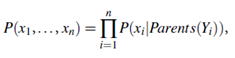
where P(x1, : : : , xn) is the probability of a particular combination of values of X, and the values for P(xi|Parents(Yi)) correspond to the entries in the CPT for Yi.

A node within the network can be selected as an “output” node, representing a class label attribute. There may be more than one output node. Various algorithms for learning can be applied to the network. Rather than returning a single class label, the classification process can return a probability distribution that gives the probability of each class.