SKEDSOFT

Introduction: Bayesian classifiers are statistical classifiers. They can predict class membership probabilities, such as the probability that a given tuple belongs to a particular class.

Bayesian classification is based on Bayes’ theorem, described below. Studies comparing classification algorithms have found a simple Bayesian classifier known as the naïve Bayesian classifier to be comparable in performance with decision tree and selected neural network classifiers. Bayesian classifiers have also exhibited high accuracy and speed when applied to large databases.

Naïve Bayesian classifiers assume that the effect of an attribute value on a given class is independent of the values of the other attributes. This assumption is called class conditional independence. It is made to simplify the computations involved and, in this sense, is considered “naïve.” Bayesian belief networks are graphical models, which unlike naïve Bayesian classifiers allow the representation of dependencies among subsets of attributes. Bayesian belief networks can also be used for classification.

Bayes’ Theorem: Bayes’ theorem is named after Thomas Bayes, a nonconformist English clergyman who did early work in probability and decision theory during the 18th century. Let X is a data tuple. In Bayesian terms, X is considered “evidence.” As usual, it is described by measurements made on a set of n attributes. Let H be some hypothesis, such as that the data tuple X belongs to a specified class C. For classification problems, we want to determine P (H|X), the probability that the hypothesis H holds given the “evidence” or observed data tuple X. In other words, we are looking for the probability that tuple X belongs to class C, given that we know the attribute description of X. P (H|X) is the posterior probability, or a posteriori probability, of H conditioned on X.

For example, suppose our world of data tuples is confined to customers described by the attributes age and income, respectively, and that X is a 35-year-old customer with an income of $40,000. Suppose that H is the hypothesis that our customer will buy a computer. Then P(H|X) reflects the probability that customer X will buy a computer given that we know the customer’s age and income.

In contrast, P(H) is the prior probability, or a priori probability, of H. For our example, this is the probability that any given customer will buy a computer, regardless of age, income, or any other information, for that matter. The posterior probability, P(H|X), is based on more information (e.g., customer information) than the prior probability, P(H), which is independent of X.

Similarly, P(X|H) is the posterior probability of X conditioned on H. That is, it is the probability that customers, X, is 35 years old and earns $40,000, given that we know the customer will buy a computer.

P(X) is the prior probability of X. Using our example, it is the probability that a person from our set of customers is 35 years old and earns $40,000.

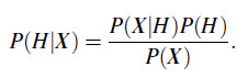
“How are these probabilities estimated?” P(H), P(X|H), and P(X) may be estimated from the given data, as we shall see below. Bayes’ theorem is useful in that it provides a way of calculating the posterior probability, P(H|X), from P(H), P(X|H), and P(X). Bayes’ theorem is

Now that we’ve got that out of the way, in the next section, we will look at how Bayes’ theorem is used in the naive Bayesian classifier.