SKEDSOFT

Introduction: A binary variable has only two states: 0 or 1, where 0 means that the variable is absent, and 1 means that it is present. Given the variable smoker describing a patient, for instance, 1 indicates that the patient smokes, while 0 indicates that the patient does not. Treating binary variables as if they are interval-scaled can lead to misleading clustering results. Therefore, methods specific to binary data are necessary for computing dissimilarities.

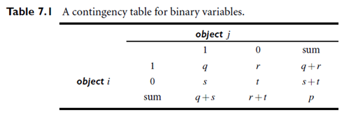
“So, how can we compute the dissimilarity between two binary variables?” One approach involves computing a dissimilarity matrix from the given binary data. If all binary variables are thought of as having the same weight, we have the 2-by-2 contingency table of Table 7.1, where q is the number of variables that equal 1 for both objects i and j, r is the number of variables that equal 1 for object i but that are 0 for object j, s is the number of variables that equal 0 for object i but equal 1 for object j, and t is the number of variables that equal 0 for both objects i and j. The total number of variables is p, where

p = q r s t.

“What is the difference between symmetric and asymmetric binary variables?” A binary variable is symmetric if both of its states are equally valuable and carry the same weight; that is, there is no preference on which outcome should be coded as 0 or 1. One such example could be the attribute gender having the states male and female. Dissimilarity that is based on symmetric binary variables is called symmetric binary dissimilarity. Its dissimilarity (or distance) measure, defined in Equation (7.9), can be used to assess the dissimilarity between objects i and j.

d(i, j) = (r s)/(q r s t)

A binary variable is asymmetric if the outcomes of the states are not equally important, such as the positive and negative outcomes of a disease test. By convention, we shall code the most important outcome, which is usually the rarest one, by 1 (e.g., HIV positive) and the other by 0 (e.g., HIV negative). Given two asymmetric binary variables, the agreement of two 1s (a positive match) is then considered more significant than that of two 0s (a negative match). Therefore, such binary variables are often considered “monary” (as if having one state). The dissimilarity based on such variables is called asymmetric binary dissimilarity, where the number of negative matches, t, is considered unimportant and thus is ignored in the computation, as shown in Equation (7.10).

d(i, j) = (r s) / (q r s)

Complementarily, we can measure the distance between two binary variables based on the notion of similarity instead of dissimilarity. For example, the asymmetric binary similarity between the objects i and j, or sim (i, j), can be computed as,

sim(i, j) = q / (q r s) = 1-d(i, j)

The coefficient sim(i, j) is called the Jaccard coefficient, which is popularly referenced in the literature.