SKEDSOFT
Introduction: Data mining often requires data integration—the merging of data from multiple data stores. The data may also need to be transformed into forms appropriate for mining. This section describes both data integration and data transformation.
Data Integration: It is likely that your data analysis task will involve data integration, which combines data from multiple sources into a coherent data store, as in data warehousing. These sources may include multiple databases, data cubes, or flat files.
There are a number of issues to consider during data integration. Schema integration and object matching can be tricky. How can equivalent real-world entities from multiple data sources be matched up? This is referred to as the entity identification problem. For example, how can the data analyst or the computer be sure that customer id in one database and cust number in another refers to the same attribute? Examples of metadata for each attribute include the name, meaning, data type, and range of values permitted for the attribute, and null rules for handling blank, zero, or null values (Section 2.3). Such metadata can be used to help avoid errors in schema integration. The metadata may also be used to help transform the data (e.g., where data codes for pay type in one database may be “H” and “S”, and 1 and 2 in another). Hence, this step also relates to data cleaning, as described earlier.
Redundancy is another important issue. An attribute (such as annual revenue, for instance) may be redundant if it can be “derived” from another attribute or set of attributes. Inconsistencies in attribute or dimension naming can also cause redundancies in the resulting data set.
Some redundancies can be detected by correlation analysis. Given two attributes, such analysis can measure how strongly one attribute implies the other, based on the available data. For numerical attributes, we can evaluate the correlation between two attributes, A and B, by computing the correlation coefficient (also known as Pearson’s product moment coefficient, named after its inventor, Karl Pearson). This is
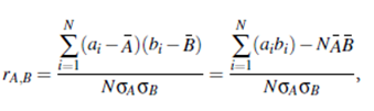
where N is the number of tuples, ai and bi are the respective values of A and B in tuple i, A and B are the respective mean values of A and B, sA and sB are the respective standard deviations of A and B (as defined in Section 2.2.2), and Σ (aibi) is the sum of the AB cross-product (that is, for each tuple, the value for A is multiplied by the value for B in that tuple).Note that -1≤rA;B ≤ 1. If rA;B is greater than 0, then A and B are positively correlated, meaning that the values of A increase as the values of B increase. The higher the value, the stronger the correlation (i.e., the more each attribute implies the other). Hence, a higher value may indicate that A (or B) may be removed as a redundancy. If the resulting value is equal to 0, then A and B are independent and there is no correlation between them. If the resulting value is less than 0, then A and B are negatively correlated, where the values of one attribute increase as the values of the other attribute decrease. This means that each attribute discourages the other. Scatter plots can also be used to view correlations between attributes (Section 2.2.3).
Note that correlation does not imply causality. That is, if A and B are correlated, this does not necessarily imply that A causes B or that B causes A. For example, in analyzing a demographic database, we may find that attributes representing the number of hospitals and the number of car thefts in a region are correlated. This does not mean that one causes the other. Both are actually causally linked to a third attribute, namely, population.
For categorical (discrete) data, a correlation relationship between two attributes, A and B, can be discovered by a c2 (chi-square) test. Suppose A has c distinct values, namely a1;a2; : : :ac. B has r distinct values, namely b1;b2; : : :br. The data tuples described by A and B can be shown as a contingency table, with the c values of A making up the columns and the r values of B making up the rows. Let (Ai;Bj) denote the event that attribute A takes on value ai and attribute B takes on value bj, that is, where (A = ai;B = bj). Each and every possible (Ai;Bj) joint event has its own cell (or slot) in the table. The c2 value (also known as the Pearson c2 statistic) is computed as:
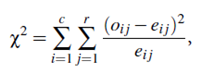
where oi j is the observed frequency (i.e., actual count) of the joint event (Ai;Bj) and ei j is the expected frequency of (Ai;Bj), which can be computed as
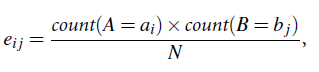
where N is the number of data tuples, count(A=ai) is the number of tuples having value ai for A, and count(B = bj) is the number of tuples having value bj for B. The sum in Equation (2.9) is computed over all of the r . c cells. Note that the cells that contribute the most to the c2 value are those whose actual count is very different from that expected.
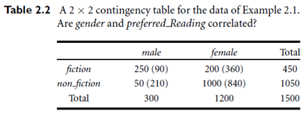
Thec2 statistic tests the hypothesis that A and B are independent. The test is based on a significance level, with (r-1)X(c-1) degrees of freedom. We will illustrate the use of this statistic in an example below. If the hypothesis can be rejected, then we say that A and B are statistically related or associated.
