SKEDSOFT

Introduction: In comparison with supervised learning, clustering lacks guidance from users or classifiers (such as class label information), and thus may not generate highly desirable clusters. The quality of unsupervised clustering can be significantly improved using some weak form of supervision, for example, in the form of pair wise constraints (i.e., pairs of objects labeled as belonging to the same or different clusters). Such a clustering process based on user feedback or guidance constraints is called semi-supervised clustering.

Methods for semi-supervised clustering can be categorized into two classes: constraint-based semi-supervised clustering and distance-based semi-supervised clustering. Constraint-based semi-supervised clustering relies on user-provided labels or constraints to guide the algorithm toward a more appropriate data partitioning. This includes modifying the objective function based on constraints, or initializing and constraining the clustering process based on the labeled objects. Distance-based semi-supervised clustering employs an adaptive distance measure that is trained to satisfy the labels or constraints in the supervised data. Several different adaptive distance measures have been used, such as string-edit distance trained using Expectation-Maximization (EM), and Euclidean distance modified by a shortest distance algorithm.

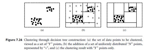
An interesting clustering method, called CL Tree (Clustering based on decision TREEs), integrates unsupervised clustering with the idea of supervised classification. It is an example of constraint-based semi-supervised clustering. It transforms a clustering task into a classification task by viewing the set of points to be clustered as belonging to one class, labeled as “Y,” and adds a set of relatively uniformly distributed, “nonexistence points” with a different class label, “N.” The problem of partitioning the data space into data (dense) regions and empty (sparse) regions can then be transformed into a classification problem. For example, Figure 7.26(a) contains a set of data points to be clustered. These points can be viewed as a set of “Y” points. Figure 7.26(b) shows the addition of a set of uniformly distributed “N” points, represented by the “o” points.  The original clustering problem is thus transformed into a classification problem, which works out a scheme that distinguishes “Y” and “N” points. A decision tree induction method can be applied to partition the two-dimensional space, as shown in Figure 7.26(c). Two clusters are identified, which are from the “Y” points only.

Adding a large number of “N” points to the original data may introduce unnecessary overhead in computation. Furthermore, it is unlikely that any points added would truly be uniformly distributed in a very high-dimensional space as this would require an exponential number of points. To deal with this problem, we do not physically add any of the “N” points, but only assume their existence. This works because the decision tree method does not actually require the points. Instead, it only needs the number of “N” points at each decision tree node. This number can be computed when needed, without having to add points to the original data. Thus, CL Tree can achieve the results in Figure 7.26(c) without actually adding any “N” points to the original data. Again, two clusters are identified.

The question then is how many (virtual) “N” points should be added in order to achieve good clustering results. The answer follows this simple rule: At the root node, the number of inherited “N” points is 0. At any current node, E, if the number of “N” points inherited from the parent node of E is less than the number of “Y” points in E, then the number of “N” points for E is increased to the number of “Y” points in E. (That is, we set the number of “N” points to be as big as the number of “Y” points.) Otherwise, the number of inherited “N” points is used in E. The basic idea is to use an equal number of “N” points to the number of “Y” points.

Decision tree classification methods use a measure, typically based on information gain, to select the attribute test for a decision node. The data are then split or partitioned according the test or “cut.” Unfortunately, with clustering, this can lead to the fragmentation of some clusters into scattered regions. To address this problem, methods were developed that use information gain, but allow the ability to look ahead.

That is, CL Tree first finds initial cuts and then looks ahead to find better partitions that cut less into cluster regions. It finds those cuts that form regions with a very low relative density. The idea is that we want to split at the cut point that may result in a big empty (“N”) region, which is more likely to separate clusters. With such tuning, CL Tree can perform high- quality clustering in high-dimensional space. It can also find subspace clusters as the decision tree method normally selects only a subset of the attributes. An interesting by-product of this method is the empty (sparse) regions, which may also be useful in certain applications.