SKEDSOFT

Introduction: “How does a Bayesian belief network learn?” In the learning or training of a belief network, a number of scenarios are possible. The network topology (or “layout” of nodes and arcs) may be given in advance or inferred from the data. The network variables may be observable or hidden in all or some of the training tuples. The case of hidden data is also referred to as missing values or incomplete data.

Several algorithms exist for learning the network topology from the training data given observable variables. The problem is one of discrete optimization. For solutions, please see the bibliographic notes at the end of this chapter. Human experts usually have a good grasp of the direct conditional dependencies that hold in the domain under analysis, which helps in network design. Experts must specify conditional probabilities for the nodes that participate in direct dependencies. These probabilities can then be used to compute the remaining probability values.

If the network topology is known and the variables are observable, then training the network is straightforward. It consists of computing the CPT entries, as is similarly done when computing the probabilities involved in naive Bayesian classification.

When the network topology is given and some of the variables are hidden, there are various methods to choose from for training the belief network. We will describe a promising method of gradient descent. For those without an advanced math background, the description may look rather intimidating with its calculus-packed formulae.

However, packaged software exists to solve these equations, and the general idea is easy to follow.

Let D be a training set of data tuples, X1, X2, . . . , X_|D|. Training the belief network means that we must learn the values of the CPT entries. Let w_{i jk} be a CPT entry for the variable Yi = y_{i j} having the parents Ui = u_ik, where w_ijk == P(Yi = yij|Ui = uik). For example, if w_{i jk} is the upper leftmost CPT entry of Figure 6.11(b), then Yi is Lung Cancer; y_{i j} is its value, “yes”; Ui lists the parent nodes of Yi, namely, {Family History, Smoker}; and u_ik lists the values of the parent nodes, namely, {“yes”, “yes”}. The w_{i jk} are viewed as weights, analogous to the weights in hidden units of neural networks (Section 6.6). The set of weights is collectively referred to as W. The weights are initialized to random probability values. A gradient descent strategy performs greedy hill-climbing. At each iteration, the weights are updated and will eventually converge to a local optimum solution.

A gradient descent strategy is used to search for the w_ijk values that best model the data, based on the assumption that each possible setting of w_ijk is equally likely. Such a strategy is iterative. It searches for a solution along the negative of the gradient (i.e., steepest descent) of a criterion function. We want to find the set of weights, W, that maximize this function. To start with, the weights are initialized to random probability values.

The gradient descent method performs greedy hill-climbing in that, at each iteration or step along the way, the algorithm moves toward what appears to be the best solution at the moment, without backtracking. The weights are updated at each iteration. Eventually, they converge to a local optimum solution.

For our problem, we maximize P_w(D)= Π^|D|_d=1 Pw(X_d). This can be done by following the gradient of ln Pw(S), which makes the problem simpler. Given the network topology and initialized w_ijk, the algorithm proceeds as follows:

1.       Compute the gradients: For each i, j, k, compute

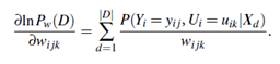
The probability in the right-hand side of Equation (6.17) is to be calculated for each training tuple, X_d, in D. For brevity, let’s refer to this probability simply as p. When the variables represented by Yi and Ui are hidden for some X_d, then the corresponding probability p can be computed from the observed variables of the tuple using standard algorithms for Bayesian network inference such as those available in the commercial software package HUGIN

2.       Take a small step in the direction of the gradient: The weights are updated by

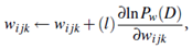
3.       Renormalize the weights: Because the weights w_ijk are probability values, they must be between 0.0 and 1.0, and Σ_j w_ijk must equal 1 for all i, k. These criteria are achieved by renormalizing the weights after they have been updated by Equation