SKEDSOFT

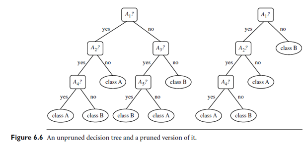
Introduction: When a decision tree is built, many of the branches will reflect anomalies in the training data due to noise or outliers. Tree pruning methods address this problem of over fitting the data. Such methods typically use statistical measures to remove the least reliable branches. An un-pruned tree and a pruned version of it are shown in Figure 6.6. Pruned trees tend to be smaller and less complex and, thus, easier to comprehend. They are usually faster and better at correctly classifying independent test data (i.e., of previously unseen tuples) than un-pruned trees.

“How does tree pruning work?” There are two common approaches to tree pruning: pre pruning and post pruning.

In the pre pruning approach, a tree is “pruned” by halting its construction early (e.g., by deciding not to further split or partition the subset of training tuples at a given node).

Upon halting, the node becomes a leaf. The leaf may hold the most frequent class among the subset tuples or the probability distribution of those tuples.

When constructing a tree, measures such as statistical significance, information gain, Gini index, and so on can be used to assess the goodness of a split. If partitioning the tuples at a node would result in a split that falls below a pre specified threshold, then further partitioning of the given subset is halted. There are difficulties, however, in choosing an appropriate threshold. High thresholds could result in oversimplified trees, whereas low thresholds could result in very little simplification.

The second and more common approach is post pruning, which removes subtrees from a “fully grown” tree. A subtree at a given node is pruned by removing its branches and replacing it with a leaf. The leaf is labeled with the most frequent class among the subtree being replaced. For example, notice the subtree at node “A3?” in the un pruned tree of Figure 6.6. Suppose that the most common class within this subtree is “class B.” In the pruned version of the tree, the sub tree in question is pruned by replacing it with the leaf “class B.”

The cost complexity pruning algorithm used in CART is an example of the post pruning approach. This approach considers the cost complexity of a tree to be a function of the number of leaves in the tree and the error rate of the tree (where the error rate is the percentage of tuples misclassified by the tree). It starts from the bottom of the tree. For each internal node, N, it computes the cost complexity of the subtree at N, and the cost complexity of the subtree at N if it were to be pruned (i.e., replaced by a leaf node). The two values are compared. If pruning the subtree at node N would result in a smaller cost complexity, then the subtree is pruned. Otherwise, it is kept. A pruning set of class-labeled tuples is used to estimate cost complexity. This set is independent of the training set used to build the un-pruned tree and of any test set used for accuracy estimation. The algorithm generates a set of progressively pruned trees. In general, the smallest decision tree that minimizes the cost complexity is preferred.

C4.5 uses a method called pessimistic pruning, which is similar to the cost complexity method in that it also uses error rate estimates to make decisions regarding subtree pruning. Pessimistic pruning, however, does not require the use of a prune set. Instead, it uses the training set to estimate error rates. Recall that an estimate of accuracy or error based on the training set is overly optimistic and, therefore, strongly biased. The pessimistic pruning method therefore adjusts the error rates obtained from the training set by adding a penalty, so as to counter the bias incurred.

Rather than pruning trees based on estimated error rates, we can prune trees based on the number of bits required to encode them. The “best” pruned tree is the one that minimizes the number of encoding bits. This method adopts the Minimum Description Length (MDL) principle, which was briefly introduced in Section 6.3.2. The basic idea is that the simplest solution is preferred. Unlike cost complexity pruning, it does not require an independent set of tuples.

Alternatively, pre pruning and post pruning may be interleaved for a combined approach. Post pruning requires more computation than pre pruning, yet generally leads to a more reliable tree. No single pruning method has been found to be superior over all others. Although some pruning methods do depend on the availability of additional data for pruning, this is usually not a concern when dealing with large databases.

Although pruned trees tend to be more compact than their un-pruned counterparts, they may still be rather large and complex. Decision trees can suffer from repetition and replication (Figure 6.7), making the mover whelming to interpret. Repetition occurs when an attribute is repeatedly tested along a given branch of the tree (such as “age < 60?”, followed by “age < 45”?, and so on). In replication, duplicate subtrees exist within the tree. These situations can impede the accuracy and comprehensibility of a decision tree. The use of multivariate splits (splits based on a combination of attributes) can prevent these problems. Another approach is to use a different form of knowledge representation, such as rules, instead of decision trees.