SKEDSOFT
Analyzing divide-and-conquer algorithms: When an algorithm contains a recursive call to itself, its running time can often be described by a recurrence equation or recurrence, which describes the overall running time on a problem of size n in terms of the running time on smaller inputs. We can then use mathematical tools to solve the recurrence and provide bounds on the performance of the algorithm.
A recurrence for the running time of a divide-and-conquer algorithm is based on the three steps of the basic paradigm. As before, we let T (n) be the running time on a problem of size n. If the problem size is small enough, say n ≤ c for some constant c, the straightforward solution takes constant time, which we write as Θ(1). Suppose that our division of the problem yields a subproblems, each of which is 1/b the size of the original. (For merge sort, both a and b are 2, but we shall see many divide-and-conquer algorithms in which a ≠ b.) If we take D(n) time to divide the problem into subproblems and C(n) time to combine the solutions to the subproblems into the solution to the original problem, we get the recurrence
![]()
Analysis of merge sort
Although the pseudocode for MERGE-SORT works correctly when the number of elements is not even, our recurrence-based analysis is simplified if we assume that the original problem size is a power of 2. Each divide step then yields two subsequences of size exactly n/2.
We reason as follows to set up the recurrence for T (n), the worst-case running time of merge sort on n numbers. Merge sort on just one element takes constant time. When we have n > 1 elements, we break down the running time as follows.
- Divide: The divide step just computes the middle of the subarray, which takes constant time. Thus, D(n) = Θ(1).
- Conquer: We recursively solve two subproblems, each of size n/2, which contributes 2T (n/2) to the running time.
- Combine: We have already noted that the MERGE procedure on an n-element subarray takes time Θ(n), so C(n) = Θ(n).
When we add the functions D(n) and C(n) for the merge sort analysis, we are adding a function that is Θ(n) and a function that is Θ(1). This sum is a linear function of n, that is, Θ(n). Adding it to the 2T (n/2) term from the "conquer" step gives the recurrence for the worst-case running time T (n) of merge sort: (2.1)
![]()
We do not need the master theorem to intuitively understand why the solution to the recurrence (2.1) is T (n) = Θ(n lg n). Let us rewrite recurrence (2.1) as
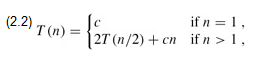
where the constant c represents the time required to solve problems of size 1 as well as the time per array element of the divide and combine steps.[8]
Figure 2.5 shows how we can solve the recurrence (2.2). For convenience, we assume that n is an exact power of 2. Part (a) of the figure shows T (n), which in part (b) has been expanded into an equivalent tree representing the recurrence. The cn term is the root (the cost at the top level of recursion), and the two subtrees of the root are the two smaller recurrences T (n/2). Part (c) shows this process carried one step further by expanding T (n/2). The cost for each of the two sub nodes at the second level of recursion is cn/2. We continue expanding each node in the tree by breaking it into its constituent parts as determined by the recurrence, until the problem sizes get down to 1, each with a cost of c. Part (d) shows the resulting tree.
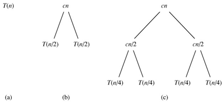
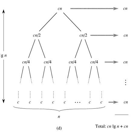
Figure 2.5: The construction of a recursion tree for the recurrence T(n) = 2T(n/2) cn. Part (a) shows T(n), which is progressively expanded in (b)-(d) to form the recursion tree. The fully expanded tree in part (d) has lg n 1 levels (i.e., it has height lg n, as indicated), and each level contributes a total cost of cn. The total cost, therefore, is cn lg n cn, which is Θ(n lg n).
- Next, we add the costs across each level of the tree. The top level has total cost cn, the next level down has total cost c(n/2) c(n/2) = cn, the level after that has total cost c(n/4) c(n/4) c(n/4) c(n/4) = cn, and so on. In general, the level i below the top has 2i nodes, each contributing a cost of c(n/2i), so that the ith level below the top has total cost 2i c(n/2i) = cn. At the bottom level, there are n nodes, each contributing a cost of c, for a total cost of cn.
- The total number of levels of the "recursion tree" in Figure 2.5 is lg n 1. This fact is easily seen by an informal inductive argument. The base case occurs when n = 1, in which case there is only one level. Since lg 1 = 0, we have that lg n 1 gives the correct number of levels. Now assume as an inductive hypothesis that the number of levels of a recursion tree for 2i nodes is lg 2i 1 = i 1 (since for any value of i, we have that lg 2i = i). Because we are assuming that the original input size is a power of 2, the next input size to consider is 2i 1. A tree with 2i 1 nodes has one more level than a tree of 2i nodes, and so the total number of levels is (i 1) 1 = lg 2i 1 1.
- To compute the total cost represented by the recurrence (2.2), we simply add up the costs of all the levels. There are lg n 1 levels, each costing cn, for a total cost of cn(lg n 1) = cn lg n cn. Ignoring the low-order term and the constant c gives the desired result of Θ(n lg n).
