SKEDSOFT

Step 1: The structure of the fastest way through the factory

• The first step of the dynamic-programming paradigm is to characterize the structure of an optimal solution. For the assembly-line scheduling problem, we can perform this step as follows. Let us consider the fastest possible way for a chassis to get from the starting point through station S_1,j. If j = 1, there is only one way that the chassis could have gone, and so it is easy to determine how long it takes to get through station S_1,j. For j = 2, 3, ..., n, however, there are two choices: the chassis could have come from station S_1,j-1 and then directly to station S_1,j, the time for going from station j - 1 to station j on the same line being negligible. Alternatively, the chassis could have come from station S_2,j-1 and then been transferred to station S_1,j, the transfer time being t_2,j-1. We shall consider these two possibilities separately, though we will see that they have much in common.
• First, let us suppose that the fastest way through station S_1,j is through station S_1,j-1. The key observation is that the chassis must have taken a fastest way from the starting point through station S_1,j-1. Why? If there were a faster way to get through station S_1,j-1, we could substitute this faster way to yield a faster way through station S_1,j: a contradiction.
• Similarly, let us now suppose that the fastest way through station S_1,j is through station S_2,j-1. Now we observe that the chassis must have taken a fastest way from the starting point through station S_2,j-1. The reasoning is the same: if there were a faster way to get through station S_2,j-1, we could substitute this faster way to yield a faster way through station S_1,j, which would be a contradiction.
• Put more generally, we can say that for assembly-line scheduling, an optimal solution to a problem (finding the fastest way through station S_i,j) contains within it an optimal solution to subproblems (finding the fastest way through either S_1,j-1 or S_2,j-1). We refer to this property as optimal substructure, and it is one of the hallmarks of the applicability of dynamic programming.

We use optimal substructure to show that we can construct an optimal solution to a problem from optimal solutions to subproblems. For assembly-line scheduling, we reason as follows. If we look at a fastest way through station S_1,j, it must go through station j - 1 on either line 1 or line 2. Thus, the fastest way through station S_1,j is either

• the fastest way through station S_1,j-1 and then directly through station S_1,j, or

• the fastest way through station S_2,j-1, a transfer from line 2 to line 1, and then through station S_1,j.

Using symmetric reasoning, the fastest way through station S_2,j is either

• the fastest way through station S_2,j-1 and then directly through station S_2,j, or

• the fastest way through station S_1,j-1, a transfer from line 1 to line 2, and then through station S_2,j.

To solve the problem of finding the fastest way through station j of either line, we solve the subproblems of finding the fastest ways through station j - 1 on both lines.

Thus, we can build an optimal solution to an instance of the assembly-line scheduling problem by building on optimal solutions to subproblems.

Step 2: A recursive solution

• The second step of the dynamic-programming paradigm is to define the value of an optimal solution recursively in terms of the optimal solutions to subproblems. For the assembly-line scheduling problem, we pick as our subproblems the problems of finding the fastest way through station j on both lines, for j = 1, 2, ..., n. Let f_i[j] denote the fastest possible time to get a chassis from the starting point through station S_i,j.

Our ultimate goal is to determine the fastest time to get a chassis all the way through the factory, which we denote by f*. The chassis has to get all the way through station n on either line 1 or line 2 and then to the factory exit. Since the faster of these ways is the fastest way through the entire factory, we have

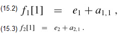
It is also easy to reason about f₁[1] and f₂[1]. To get through station 1 on either line, a chassis just goes directly to that station. Thus,

Now let us consider how to compute f_i[j] for j = 2, 3, ..., n (and i = 1, 2). Focusing on f₁[j], we recall that the fastest way through station S_1,j is either the fastest way through station S_1,j-1 and then directly through station S_1,j, or the fastest way through station S_2,j-1, a transfer from line 2 to line 1, and then through station S_1,j. In the first case, we have f₁[j] = f₁[j - 1] a_1,j, and in the latter case, f₁[j] = f₂[j - 1] t_2,j-1 a_1,j. Thus,