SKEDSOFT

Overlapping subproblems

The second ingredient that an optimization problem must have for dynamic programming to be applicable is that the space of subproblems must be "small" in the sense that a recursive algorithm for the problem solves the same subproblems over and over, rather than always generating new subproblems. Typically, the total number of distinct subproblems is a polynomial in the input size. When a recursive algorithm revisits the same problem over and over again, we say that the optimization problem has overlapping subproblems. In contrast, a problem for which a divide-and-conquer approach is suitable usually generates brand-new problems at each step of the recursion. Dynamic-programming algorithms typically take advantage of overlapping subproblems by solving each subproblem once and then storing the solution in a table where it can be looked up when needed, using constant time per lookup.

To illustrate the overlapping-subproblems property in greater detail, let us reexamine the matrix-chain multiplication problem. Referring back to Figure 15.3, observe that MATRIX-CHAIN-ORDER repeatedly looks up the solution to subproblems in lower rows when solving subproblems in higher rows. For example, entry m[3, 4] is referenced 4 times: during the computations of m[2, 4], m[1, 4], m[3, 5], and m[3, 6]. If m[3, 4] were recomputed each time, rather than just being looked up, the increase in running time would be dramatic. To see this, consider the following (inefficient) recursive procedure that determines m[i, j], the minimum number of scalar multiplications needed to compute the matrix-chain product A_i‥j = A_iA_{i 1} ··· A_j. The procedure is based directly on the recurrence (15.12).

	RECURSIVE-MATRIX-CHAIN(p, i, j)
1 if i = j
2     then return 0
3 m[i, j] ← ∞
4 for k ← i to j - 1
5      do q ← RECURSIVE-MATRIX-CHAIN(p, i, k)
                   RECURSIVE-MATRIX-CHAIN(p,k   1, j)
                   pi-1 pk pj
6         if q < m[i, j]
7            then m[i, j] ← q
8 return m[i, j]

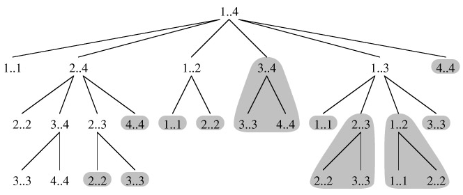
Figure 15.5 shows the recursion tree produced by the call RECURSIVE-MATRIX-CHAIN(p, 1, 4). Each node is labeled by the values of the parameters i and j. Observe that some pairs of values occur many times.

In fact, we can show that the time to compute m[1, n] by this recursive procedure is at least exponential in n. Let T (n) denote the time taken by RECURSIVE-MATRIX-CHAIN to compute an optimal parenthesization of a chain of n matrices. If we assume that the execution of lines 1-2 and of lines 6-7 each take at least unit time, then inspection of the procedure yields the recurrence

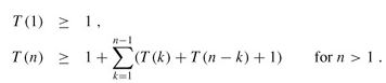
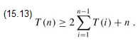
Noting that for i = 1, 2, ..., n - 1, each term T (i) appears once as T (k) and once as T (n - k), and collecting the n - 1 1's in the summation together with the 1 out front, we can rewrite the recurrence as

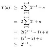
We shall prove that T (n) = Ω(2ⁿ) using the substitution method. Specifically, we shall show that T (n) ≥ 2^n-1 for all n ≥ 1. The basis is easy, since T (1) ≥ 1 = 2⁰. Inductively, for n ≥ 2 we have