SKEDSOFT

• From a theoretical standpoint, Fibonacci heaps are especially desirable when the number of EXTRACT-MIN and DELETE operations is small relative to the number of other operations performed. This situation arises in many applications. For example, some algorithms for graph problems may call DECREASE-KEY once per edge. For dense graphs, which have many edges, the O(1) amortized time of each call of DECREASE-KEY adds up to a big improvement over the Θ(lg n) worst-case time of binary or binomial heaps. Fast algorithms for problems such as computing minimum spanning trees and finding single-source shortest paths make essential use of Fibonacci heaps.
• From a practical point of view, however, the constant factors and programming complexity of Fibonacci heaps make them less desirable than ordinary binary (or k-ary) heaps for most applications. Thus, Fibonacci heaps are predominantly of theoretical interest. If a much simpler data structure with the same amortized time bounds as Fibonacci heaps were developed, it would be of practical use as well.
• Like a binomial heap, a Fibonacci heap is a collection of trees. Fibonacci heaps, in fact, are loosely based on binomial heaps. If neither DECREASE-KEY nor DELETE is ever invoked on a Fibonacci heap, each tree in the heap is like a binomial tree. Fibonacci heaps have a more relaxed structure than binomial heaps, however, allowing for improved asymptotic time bounds. Work that maintains the structure can be delayed until it is convenient to perform.
• The exposition in this chapter assumes that you have read binomial heaps. The specifications for the operations appear in that chapter, as does the table in Figure 19.1, which summarizes the time bounds for operations on binary heaps, binomial heaps, and Fibonacci heaps. Our presentation of the structure of Fibonacci heaps relies on that of binomial-heap structure, and some of the operations performed on Fibonacci heaps are similar to those performed on binomial heaps.
• Like binomial heaps, Fibonacci heaps are not designed to give efficient support to the operation SEARCH; operations that refer to a given node therefore require a pointer to that node as part of their input. When we use a Fibonacci heap in an application, we often store a handle to the corresponding application object in each Fibonacci-heap element, as well as a handle to corresponding Fibonacci-heap element in each application object.

Structure of Fibonacci heaps: Like a binomial heap, a Fibonacci heap is a collection of min-heap-ordered trees. The trees in a Fibonacci heap are not constrained to be binomial trees, however. Figure 20.1(a) shows an example of a Fibonacci heap.

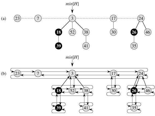
Unlike trees within binomial heaps, which are ordered, trees within Fibonacci heaps are rooted but unordered. As Figure 20.1(b) shows, each node x contains a pointer p[x] to its parent and a pointer child[x] to any one of its children. The children of x are linked together in a circular, doubly linked list, which we call the child list of x. Each child y in a child list has pointers left[y] and right[y] that point to y's left and right siblings, respectively. If node y is an only child, then left[y] = right[y] = y. The order in which siblings appear in a child list is arbitrary.

Circular, doubly linked lists have two advantages for use in Fibonacci heaps. First, we can remove a node from a circular, doubly linked list in O(1) time. Second, given two such lists, we can concatenate them (or "splice" them together) into one circular, doubly linked list in O(1) time. In the descriptions of Fibonacci heap operations, we shall refer to these operations informally, letting the reader fill in the details of their implementations.

Two other fields in each node will be of use. The number of children in the child list of node x is stored in degree[x]. The boolean-valued field mark[x] indicates whether node x has lost a child since the last time x was made the child of another node. Newly created nodes are unmarked, and a node x becomes unmarked whenever it is made the child of another node.

A given Fibonacci heap H is accessed by a pointer min[H] to the root of a tree containing a minimum key; this node is called the minimum node of the Fibonacci heap. If a Fibonacci heap H is empty, then min[H] = NIL.

The roots of all the trees in a Fibonacci heap are linked together using their left and right pointers into a circular, doubly linked list called the root list of the Fibonacci heap. The pointer min[H] thus points to the node in the root list whose key is minimum. The order of the trees within a root list is arbitrary.

We rely on one other attribute for a Fibonacci heap H: the number of nodes currently in H is kept in n[H].