SKEDSOFT

hus, we can compute the Θ(n²) values of w[i, j] in Θ(1) time each.

The pseudocode that follows takes as inputs the probabilities p₁, ..., p_n and q₀, ..., q_n and the size n, and it returns the tables e and root.

	OPTIMAL-BST(p, q, n)
 1  for i ← 1 to n   1
 2       do e[i, i - 1] ← qi-1
 3          w[i, i - 1] ← qi-1
 4  for l ← 1 to n
 5       do for i ← 1 to n - l   1
 6               do j ← i   l - 1
 7                  e[i, j] ← ∞
 8                  w[i, j] ← w[i, j - 1]   pj   qj
 9                  for r ← i to j
10                       do t ← e[i, r - 1]   e[r   1, j]   w[i, j]
11                          if t < e[i, j]
12                             then e[i, j] ← t
13                                  root[i, j] ← r
14  return e and root

From the description above and the similarity to the MATRIX-CHAIN-ORDER procedure in Section 15.2, the operation of this procedure should be fairly straightforward. The for loop of lines 1-3 initializes the values of e[i, i - 1] and w[i, i - 1]. The for loop of lines 4-13 then uses the recurrences (15.19) and (15.20) to compute e[i, j] and w[i, j] for all 1 ≤ i ≤ j ≤ n. In the first iteration, when l = 1, the loop computes e[i, i] and w[i, i] for i = 1, 2, ..., n. The second iteration, with l = 2, computes e[i, i 1] and w[i, i 1] for i = 1, 2, ..., n - 1, and so forth. The innermost for loop, in lines 9-13, tries each candidate index r to determine which key k_r to use as the root of an optimal binary search tree containing keys k_i, ..., k_j. This for loop saves the current value of the index r in root[i, j] whenever it finds a better key to use as the root.

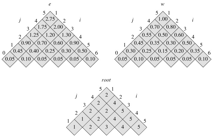
Figure 15.8 shows the tables e[i, j], w[i, j], and root[i, j] computed by the procedure OPTIMAL-BST on the key distribution shown in Figure 15.7. As in the matrix-chain multiplication example, the tables are rotated to make the diagonals run horizontally. OPTIMAL-BST computes the rows from bottom to top and from left to right within each row.

The OPTIMAL-BST procedure takes Θ(n³) time, just like MATRIX-CHAIN-ORDER. It is easy to see that the running time is O(n³), since its for loops are nested three deep and each loop index takes on at most n values. The loop indices in OPTIMAL-BST do not have exactly the same bounds as those in MATRIX-CHAIN-ORDER, but they are within at most 1 in all directions. Thus, like MATRIX-CHAIN-ORDER, the OPTIMAL-BST procedure takes Ω(n³) time.