SKEDSOFT

Figure 30.1 shows this strategy graphically. One minor detail concerns degree-bounds. The product of two polynomials of degree-bound n is a polynomial of degree-bound 2n. Before evaluating the input polynomials A and B, therefore, we first double their degree-bounds to 2n by adding n high-order coefficients of 0. Because the vectors have 2n elements, we use "complex (2n)th roots of unity," which are denoted by the w_2n terms in Figure 30.1.

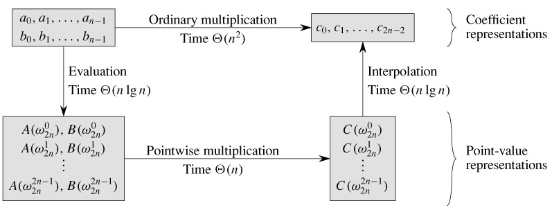
Figure 30.1: A graphical outline of an efficient polynomial-multiplication process. Representations on the top are in coefficient form, while those on the bottom are in point-value form. The arrows from left to right correspond to the multiplication operation. The w_2n terms are complex (2n)th roots of unity.

Given the FFT, we have the following Θ(n lg n)-time procedure for multiplying two polynomials A(x) and B(x) of degree-bound n, where the input and output representations are in coefficient form. We assume that n is a power of 2; this requirement can always be met by adding high-order zero coefficients.

1. Double degree-bound: Create coefficient representations of A(x) and B(x) as degree-bound 2n polynomials by adding n high-order zero coefficients to each.

2. Evaluate: Compute point-value representations of A(x) and B(x) of length 2n through two applications of the FFT of order 2n. These representations contain the values of the two polynomials at the (2n)th roots of unity.

3. Pointwise multiply: Compute a point-value representation for the polynomial C(x) = A(x)B(x) by multiplying these values together pointwise. This representation contains the value of C(x) at each (2n)th root of unity.

4. Interpolate: Create the coefficient representation of the polynomial C(x) through a single application of an FFT on 2n point-value pairs to compute the inverse DFT.

Steps (1) and (3) take time Θ(n), and steps (2) and (4) take time Θ(n lg n). Thus, once we show how to use the FFT, we will have proven the following.