SKEDSOFT

Some Applications of Special Types of Graphs: We conclude this section by introducing some additional graph models that involve the special types of graph we have discussed in this section.

EXAMPLE 1 Local Area Networks The various computers in a building, such as minicomputers and personal computers, as well as peripheral devices such as printers and plotters, can be connected using a local area network. Some of these networks are based on a star topology, where all devices are connected to a central control device.A local area network can be represented using a complete bipartite graph K1,n, as shown in Figure 11(a). Messages are sent from device to device through the central control device.

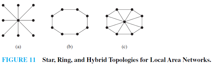
Other local area networks are based on a ring topology, where each device is connected to exactly two others. Local area networks with a ring topology are modeled using n-cycles, Cn, as shown in Figure 11(b). Messages are sent from device to device around the cycle until the intended recipient of a message is reached.

Finally, some local area networks use a hybrid of these two topologies. Messages may be sent around the ring, or through a central device. This redundancy makes the network more reliable. Local area networks with this redundancy can be modeled using wheels Wn, as shown in Figure 11(c).

EXAMPLE 2 Interconnection Networks for Parallel Computation For many years, computers executed programs one operation at a time. Consequently, the algorithms written to solve problems were designed to perform one step at a time; such algorithms are called serial. (Almost all algorithms described in this book are serial.) However, many computationally intense problems, such as weather simulations, medical imaging, and cryptanalysis, cannot be solved in a reasonable amount of time using serial operations, even on a supercomputer. Furthermore, there is a physical limit to how fast a computer can carry out basic operations, so there will always be problems that cannot be solved in a reasonable length of time using serial operations.

Parallel processing, which uses computers made up of many separate processors, each with its own memory, helps overcome the limitations of computers with a single processor. Parallel algorithms, which break a problem into a number of subproblems that can be solved

concurrently, can then be devised to rapidly solve problems using a computer with multiple processors. In a parallel algorithm, a single instruction stream controls the execution of the algorithm, sending subproblems to different processors, and directs the input and output of these subproblems to the appropriate processors.

When parallel processing is used, one processor may need output generated by another processor. Consequently, these processors need to be interconnected.We can use the appropriate type of graph to represent the interconnection network of the processors in a computer with multiple processors. In the following discussion, we will describe the most commonly used types of interconnection networks for parallel processors. The type of interconnection network used to implement a particular parallel algorithm depends on the requirements for exchange of data between processors, the desired speed, and, of course, the available hardware.

The simplest, but most expensive, network-interconnecting processors include a two-way link between each pair of processors. This network can be represented by Kn, the complete graph on n vertices, when there are n processors. However, there are serious problems with this type of interconnection network because the required number of connections is so large. In reality, the number of direct connections to a processor is limited, so when there are a large number of processors, a processor cannot be linked directly to all others. For example, when there are 64 processors, C(64, 2) = 2016 connections would be required, and each processor would have to be directly connected to 63 others.

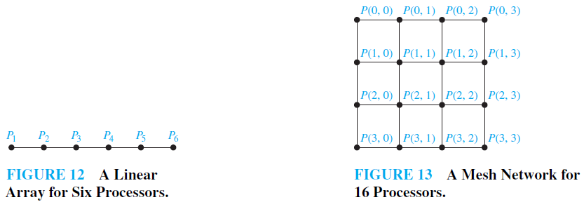
On the other hand, perhaps the simplest way to interconnect n processors is to use an arrangement known as a linear array. Each processor Pi , other than P1 and Pn, is connected to its neighbors P_i−1 and P_{i 1} via a two-way link. P1 is connected only to P2, and Pn is connected only to Pn−1. The linear array for six processors is shown in Figure 12. The advantage of a linear array is that each processor has at most two direct connections to other processors. The disadvantage is that it is sometimes necessary to use a large number of intermediate links, called hops, for processors to share information.

The mesh network (or two-dimensional array) is a commonly used interconnection network. In such a network, the number of processors is a perfect square, say n = m2. The n processors are labeled P(i, j), 0 ≤ i ≤ m − 1, 0 ≤ j ≤ m − 1. Two-way links connect processor P(i, j) with its four neighbors, processors P(i ± 1, j) and P(i, j ± 1), as long as these are processors in the mesh. The mesh network limits the number of links for each processor. Communication between some pairs of processors requires O( √ n) = O(m) intermediate links. The graph representing the mesh network for 16 processors is shown in Figure 13.

One important type of interconnection network is the hypercube. For such a network, the number of processors is a power of 2, n = 2m. The n processors are labeled P0, P1, . . . , Pn−1. Each processor has two-way connections to m other processors. Processor Pi is linked to the processors with indices whose binary representations differ from the binary representation of i in exactly one bit. The hypercube network balances the number of direct connections for each processor and the number of intermediate connections required so that processors can communicate. Many computers have been built using a hypercube network, and many parallel algorithms have been devised that use a hypercube network. The graph Qm, the m-cube, represents the hypercube network with n = 2m processors. Figure 14 displays the hypercube network for eight processors.