SKEDSOFT
Curve Tracing:
The elementary method of tracing (or plotting) a curve whose equation is given in rectangular coordinates, and one with which the student is already familiar, is to solve its equation for y (or y ), assume arbitrary values of y (or y ), calculate the corresponding values of y (or y ), plot the respective points, and draw a smooth curve through them, the result being an approximation to the required curve. This process is laborious at best, and in case the equation of the curve is of a degree higher than the second, the solved form of such an equation may be unsuitable for the purpose of computation, or else it may fail altogether, since it is not always possible to solve the equation for y or y. The general form of a curve is usually all that is desired, and the Calculus furnishes us with powerful methods for determining the shape of a curve with very little computation. The first derivative gives us the slope of the curve at any point; the second derivative determines the intervals within which the curve is concave upward or concave downward, and the points of inflection separate these intervals; the maximum points are the high points and the minimum points are the low points on the curve. As a guide in his work the student may follow:
Rule for tracing curves. Rectangular Coordinates:
- FIRST STEP: Find the first derivative; place it equal to zero; solving gives the abscissas of maximum and minimum points.
- SECOND STEP: Find the second derivative; place it equal to zero; solving gives the abscissas of the points of inflection.
- THIRD STEP: Calculate the corresponding ordinates of the points whose abscissas were found in the first two steps. Calculate as many more points as may be necessary to give a good idea of the shape of the curve. Fill out a table such as is shown in the example worked out.
- FOURTH STEP: Plot the points determined and sketch in the curve to correspond with the results shown in the table.
If the calculated values of the ordinates are large, it is best to reduce the scale on the y-axis so that the general behavior of the curve will be shown within the limits of the paper used. Coordinate plotting (graph) paper should be employed.
Pricipal Curve:
Let x ∈ Rn be a random vector with samples x1,x2,........,xN having a given PDF estimate of p(x). Let g(x) be the transpose of its local gradient and let H(x) be the local Hessian of this pdf. Finally using the gradient and Hessian define the local convariance as: 
Let  be the eigen value and vector pairs of
  sorted in ascending order
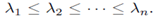
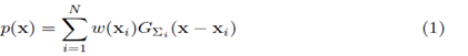
Where w (xi) is the weight and  is the variable kernel convariance of the Gaussian Kernal
 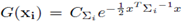 . The gradient and the Hessian of the KDE are:
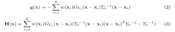
For p(x) mean shift update are in the form of 

Hence this is the basic Pricipal of Curve Tracing Methods.
