SKEDSOFT
Curve Fitting:
The curve fitting process fits the equation of approximating curves to the raw field data. Nevertheless, for a given set of data, the fitting curves of a given type are generally NOT unique. Thus, a curve with a minimal deviation from all data points is desired.
The Method of Least Squares:
Principle of Least Square: The curve of best fit is that for which the sum of squares of the residuals is minimum. The method of least squares assumes that the best-fit curve of a given type is the curve that has the minimal sum of the deviations squared (least square error) from a given set of data. Let the set of data points be (xi, yi), i = 1,2, ...,m, and let the curve given by y = f (x) be fitted to this data. At x = xi, the observed value of the ordinate is yi and the corresponding value on the fitting curve is f (xi). If εi is the error of approximation at x = xi, then we have
εi = yi− f (xi)
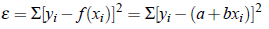
The sum of square of errors,
ε = Σei 2 = Σ[yi− f (xi)]2
Now if ε = 0 then yi = f (xi), i.e. all the points lie on the curve. Otherwise, the minimum e results the best fitting of the curve to the data.
Fitting of A Straight Line:
Let (xi, yi) be n sets of observations of related data and y = a bx be the straight line to be fitted.Then equation
By the principle of least square, ε is minimum for some a and b, i.e.,
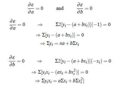
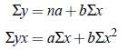
These above equations are called normal equations. Since xi and yi are known, these equations result in equations in a and b. We can solve these for a and b.
Remark: For the sake of simplicity leave suffix notation to obtain the following form of normal equations.