SKEDSOFT

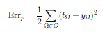
Introduction:-The learning curve indicates the progress of the error, which can be determined in various ways. The motivation to create a learning curve is that such a curve can indicate whether the network is progressing or not. For this, the error should be normalized i.e. represent a distance measure between the correct and the current output of the network. For example, we can take the same pattern specific, squared error with a prefactor, which we are also going to use to derive the backpropagation of error (let be output neurons and other set of output neurons:-

Specific error Errp is based on a single Errp training sample, which means it is generated online. Additionally, the root mean square (abbreviated:RMS) and the Euclideandistance are often used. The Euclidean distance (generalization other theorem of Pythagoras) is useful for lower dimensions where we can still visualize its usefulness.

The Euclidean distance between two vectors t and y is defined as

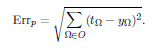
Generally, the root mean square is commonly used since it considers extreme outliers to a greater extent.As for offline learning, the total error in the course of one training epoch is interesting and useful too:

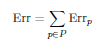
The total error Err is based on all training samples, that means it is generated offline.

Analogously we can generate a total RMS and a total Euclidean distance in the course of a whole epoch. Of course, it is possible to use other types of error measurement.To get used to further error measurement methods, I suggest to have a look into the technical report of Prechelt. Depending on our method of error measurement our learning curve certainlychanges, too. A perfect learning curve looks like a negative exponential function. Thus the representation of the learning curve can be illustrated by means of a logarithmic scale with the said scaling combination a descending line implies an exponential descent of the error. With the network doing a good job, the problems being not too difficult and the

logarithmic representation of Err you can see - metaphorically speaking - a descending line that often forms "spikes" at the bottom – here, we reach the limit of the 64-bit resolution of our computer and our network has actually learned the optimum of what it is capable of learning. Typical learning curves can show a few flat areas as well, i.e. they can show some steps, which is no sign of a malfunctioning learning process. A well-suited representation can make any slightly decreasing learning curve look good.