SKEDSOFT
Wave equation :The Wave equation is swecond order linear partial differentiation for discription of wave such as light and sound waves.
The linear second order partial differential equation is given by,

as an hyperbolic equation if B2 – AC > 0. An hyperbolic equation holds in an open domain or in a semi-open domain. The simplest example of an hyperbolic equation is the one dimensional wave equation.
Study of the behavior of waves is one of the important areas in engineering. All vibration problems are governed by wave equations.
Consider the problem of a vibrating elastic string of length l, located on the x-axis on the interval [0, l]. Let u(x, t) denote the displacement of the string in the vertical plane. Then, the vibrations of the elastic string is governed by the one dimensional wave equation.
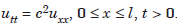 ...................1.1
where c2 is a constant and depends on the material properties of the string, the tension T in the string and the mass per unit length of the string.
In order that the solution of the problem exists and is unique, we need to prescribe the following conditions.
(i) Initial condition Displacement at time t = 0 or initial displacement is given by u(x, 0) = f(x), 0 ≤ x ≤ l. Initial velocity: ut(x, 0) = g(x), 0 ≤ x ≤ l. (5.53 b)
(ii) Boundary conditions We consider the case when the ends of the string are fixed. Since the ends are fixed, we have the boundary conditions as
u(0, t) = 0, u(l, t) = 0, t > 0. (5.53)
Since both the initial and boundary conditions are prescribed, the problem is called an initial boundary value problem.
Mesh generation : The mesh is generated as in the case of the heat conduction equation. Superimpose on the region 0 ≤ x ≤ l, t > 0, a rectangular network of mesh lines. Let the interval [0, l] be divided into M parts. Then, the mesh length along the x-axis is h = l/M. The points along the xaxis are xi = ih, i = 0, 1, 2, ..., M. Let the mesh length along the t-axis be k and define tj = jk. The mesh points are (xi , tj) . We call tj as the jth time level. At any point (xi , tj), we denote the numerical solution by ui, j and the exact solution by u(xi , tj).
