SKEDSOFT

This method is also known as Guassian integration rule or guassian formula.In this case the weight function is w(x) = 1,

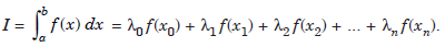
Since the weight function is w(x) = 1, we shall write the integration rule as

..............1.1

As mentioned earlier, the limits of integration for Gauss-Legendre integration rules are [– 1, 1]. Therefore, we transform the limits [a, b] to [– 1, 1], using a linear transformation.

Let the transformation be x = pt q.

When x = a, we have t = – 1: a = – p q.

When x = b, we have t = 1: b = p q.

Solving, we get p(b – a)/2, q = (b a)/2.

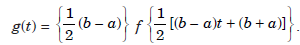
The required transformation is

                                                                                         x = 1/2 [(b – a)t (b a)]. ......................1.2

Then,

f(x) = f{[(b – a)t (b a)]/2} and dx = [(b – a)/2]dt.

The integral becomes

.....................1.3

where,

Therefore, we shall derive formulas to evaluate

Without loss of generality, let us write this integral as

The required integration formula is of the form

.....................1.4

Before deriving the methods, let us remember the definition of the order of a method and the expression for the error of the method.

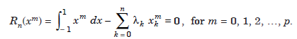
An integration method of the form (1.4) is said to be of order p, if it produces exact results, that is error R_n = 0, for all polynomials of degree less than or equal to p.

That is, it produces exact results for f(x) = 1, x, x², ..., x^p. When w(x) = 1, this implies that

The error term is obtained for f(x) = x^{p 1}. We define

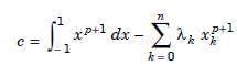....................1.5