SKEDSOFT

Introduction :

Consider a system of n linear algebraic equations in n unknowns

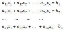
where a_ij, i = 1, 2, ..., n, j = 1, 2, …, n, are the known coefficients, b_i , i = 1, 2, …, n, are the know right hand side values and x_i, i = 1, 2, …, n are the unknowns to be determined.

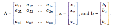
In matrix notation we write the system as

Ax = b...................1.1

where,

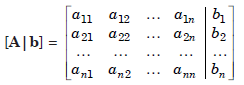
The matrix [A | b], obtained by appending the column b to the matrix A is called the augmented matrix.

That is,

We define the following,

(i) The system of equations (1.1) is consistent (has at least one solution), if

rank (A) = rank [A | b] = r.

If r = n, then the system has unique solution.

If r < n, then the system has (n – r) parameter family of infinite number of solutions.

(ii) The system of equations (1.1) is inconsistent (has no solution) if

                                                                                                                         rank (A) ≠ rank [A | b].

We assume that the given system is consistent.
The methods of solution of the linear algebraic system of equations (1.1) may be classified as direct and iterative methods.

(a) Direct methods produce the exact solution after a finite number of steps (disregarding the round-off errors). In these methods, we can determine the total number of operations (additions, subtractions, divisions and multiplications). This number is called the operational count of the method.

(b) Iterative methods are based on the idea of successive approximations. We start with an initial approximation to the solution vector x = x₀, and obtain a sequence of approximate vectors x₀, x₁, ..., x_k, ..., which in the limit as k → ∞, converge to the exact solution vector x.