SKEDSOFT

Runge Kutta Methods: A method of numerically integrating ordinary differential equations by using a trial step at the midpoint of an interval to cancel out lower-order error terms

Integrating the differential equation y′ = f (x, y) in the interval [x_i, x_{i 1}], we get

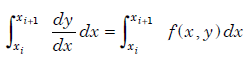.........................1.1

We have noted in the previous section, that y′ and hence f (x, y) is the slope of the solution curve. Further, the integrand on the right hand side is the slope of the solution curve which changes continuously in [x_i, x_{i 1}]. By approximating the continuously varying slope in [x_i, x_{i 1}] by a fixed slope, we have obtained the Euler, Heun’s and modified Euler methods. The basic idea of Runge-Kutta methods is to approximate the integral by a weighted average of slopes and approximate slopes at a number of points in [x_i, x_{i 1}]. If we also include the slope at x_{i 1}, we obtain implicit Runge-Kutta methods. If we do not include the slope at x_{i 1}, we obtain explicit Runge-Kutta methods. For our discussion, we shall consider explicit Runge-Kutta methods only. However, Runge-Kutta methods must compare with the Taylor series method when they are expanded about the point x = x_i. In all the Runge-Kutta methods, we include the slope at the initial point x = x_i, that is, the slope f(x_i, y_i).

Runge-Kutta method of second order :

Consider a Runge-Kutta method with two slopes. Define

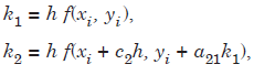
.......................1.1

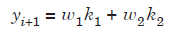
where the values of the parameters c₂, a₂₁, w₁, w₂ are chosen such that the method is of highest possible order. Now, Taylor series expansion about x = x_i, gives

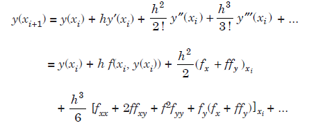....................1.2

We also have,

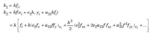
Substituting the values of k₁ and k₂ in (1.2), we get,

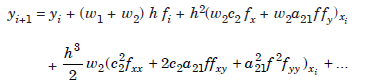.................1.3