SKEDSOFT

Stability of Numericals Method :   This section gives the stability of different numericals methods.

1.  In any initial value problem, we require solution for x > x0 and usually up to a point x = b. The step length h for application of any numerical method for the initial value problem must be properly chosen.

2.  The computations contain mainly two types of errors: truncation error and round-off error.

3.  Truncation error is in the hand of the user. It can be controlled by choosing higher order methods.

4.  Round-off errors are not in the hands of the user. They can grow and finally destroy the true solution.

5.  In such case, we say that the method is numerically unstable. This happens when the step length is chosen larger than the allowed limiting value.

6.  All explicit methods have restrictions on the step length that can be used.

7.  Many implicit methods have no restriction on the step length that can be used. Such methods are called unconditionally stable methods.

The behaviour of the solution of the given initial value problem is studied by considering the linearized form of the differential equation y′ = f (x, y). The linearized form of the initial value problem is given by y′ = λ y, λ < 0, y(x₀) = y₀. The single step methods are applied to this differential equation to obtain the difference equation y_{i 1} = E(λh)y_i, where E(λh) is called the amplification factor. If | E(λh) | < 1, then all the errors (round-off and other errors) decay and the method gives convergent solutions. We say that the method is stable. This condition gives a bound on the step length h that can be used in the computations. We have the following conditions for stability of the single step methods that are considered in the previous sections.

1. Euler method: – 2 < λh < 0.

2. Runge-Kutta method of second order: – 2 < λh < 0.

3. Classical Runge-Kutta method of fourth order: – 2.78 < λh < 0.

4. Backward Euler method: Stable for all h, that is, – ∞ < λh < 0. (Unconditionally stable method).

Similar stability analysis can be done for the multi step methods. We have the following stability intervals (condition on λ h), for the multi step methods that are considered in the previous sections.

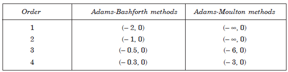
Thus, we conclude that a numerical method can not be applied as we like to a given initial value problem. The choice of the step length is very important and it is governed by the stability condition.

For example, if we are solving the initial value problem y′ = – 100y, y(x₀) = y₀, by Euler method, then the step length should satisfy the condition – 2 < λh < 0 or – 2 < – 100h < 0, or h < 0.02.

The predictor-corrector methods also have such strong stability conditions.