SKEDSOFT

PRIORITY-DRIVEN APPROACH: The term priority-driven algorithms refers to a large class of scheduling algorithms that never leave any resource idle intentionally. Stated in another way, a resource idles only when no job requiring the resource is ready for execution. Scheduling decisions are made when events such as releases and completions of jobs occur. Hence, priority-driven algorithms are event-driven.

Other commonly used names for this approach are greedy scheduling, list scheduling and work-conserving scheduling. A priority-driven algorithm is greedy because it tries to make locally optimal decisions. Leaving a resource idle while some job is ready to use the resource is not locally optimal. So when a processor or resource is available and some job can use it to make progress, such an algorithm never makes the job wait. We will return shortly to illustrate that greed does not always pay; sometimes it is better to have some jobs wait even when they are ready to execute and the resources they require are available.

The term list scheduling is also descriptive because any priority-driven algorithm can be implemented by assigning priorities to jobs. Jobs ready for execution are placed in one or more queues ordered by the priorities of the jobs. At any scheduling decision time, the jobs with the highest priorities are scheduled and executed on the available processors. Hence, a priority-driven scheduling algorithm is defined to a great extent by the list of priorities it assigns to jobs; the priority list and other rules, such as whether preemption is allowed, define the scheduling algorithm completely.

Most scheduling algorithms used in nonreal-time systems are priority-driven. Examples include the FIFO (First-In-First-Out) and LIFO (Last-In-First-Out) algorithms, which assign priorities to jobs according their release times, and the SETF (Shortest-Execution-Time-First) and LETF (Longest-Execution-Time-First) algorithms, which assign priorities on the basis of job execution times. Because we can dynamically change the priorities of jobs, even roundrobin scheduling can be thought of as priority-driven: The priority of the executing job is lowered to the minimum among all jobs waiting for execution after the job has executed for a time slice.

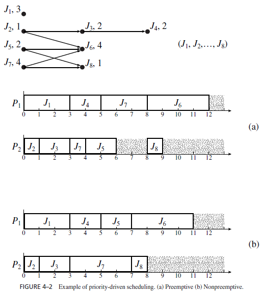
Figure 4–2 gives an example. The task graph shown here is a classical precedence graph; all its edges represent precedence constraints. The number next to the name of each job is its execution time. J5 is released at time 4. All the other jobs are released at time 0. We want to schedule and execute the jobs on two processors P1 and P2. They communicate via a shared memory. Hence the costs of communication among jobs are negligible no matter where they are executed. The schedulers of the processors keep one common priority queue of ready jobs. The priority list is given next to the graph: Ji has a higher priority than Jk if i < k. All the jobs are preemptable; scheduling decisions are made whenever some job becomes ready for execution or some job completes.

Figure 4–2(a) shows the schedule of the jobs on the two processors generated by the priority-driven algorithm following this priority assignment. At time 0, jobs J1, J2, and J7 are ready for execution. They are the only jobs in the common priority queue at this time. Since J1 and J2 have higher priorities than J7, they are ahead of J7 in the queue and hence are scheduled. The processors continue to execute the jobs scheduled on them except when the following events occur and new scheduling decisions are made.

• At time 1, J2 completes and, hence, J3 becomes ready. J3 is placed in the priority queue ahead of J7 and is scheduled on P2, the processor freed by J2.
• At time 3, both J1 and J3 complete. J5 is still not released. J4 and J7 are scheduled.
• At time 4, J5 is released. Now there are three ready jobs. J7 has the lowest priority among them. Consequently, it is preempted. J4 and J5 have the processors.
• At time 5, J4 completes. J7 resumes on processor P1.
• At time 6, J5 completes. Because J7 is not yet completed, both J6 and J8 are not ready for execution. Consequently, processor P2 becomes idle.
• J7 finally completes at time 8. J6 and J8 can now be scheduled and they are.

Figure 4–2(b) shows a nonpreemptive schedule according to the same priority assignment. Before time 4, this schedule is the same as the preemptive schedule. However, at time 4 when J5 is released, both processors are busy. It has to wait until J4 completes (at time 5) before it can begin execution. It turns out that for this system this postponement of the higher priority job benefits the set of jobs as a whole. The entire set completes 1 unit of time earlier according to the nonpreemptive schedule.

In general, however, nonpreemptive scheduling is not better than preemptive scheduling. A fundamental question is, when is preemptive scheduling better than nonpreemptive scheduling and vice versa? It would be good if we had some rule with which we could determine from the given parameters of the jobs whether to schedule them preemptively or nonpreemptively. Unfortunately, there is no known answer to this question in general. In the special case when jobs have the same release time, preemptive scheduling is better when the cost of preemption is ignored.

Specifically, in a multiprocessor system, the minimum makespan (i.e., the response time of the job that completes last among all jobs) achievable by an optimal preemptive algorithm is shorter than the makespan achievable by an optimal nonpreemptive algorithm. A natural question here is whether the difference in the minimum makespans achievable by the two classes of algorithms is significant, in particular, whether the theoretical gain in makespan achievable by preemption is enough to compensate for the context switch overhead of preemption. The answer to this question is only known for the two-processor case. Coffman and Garey [CoGa] recently proved that when there are two processors, the minimum makespan achievable by nonpreemptive algorithms is never more than 4/3 times the minimum makespan achievable by preemptive algorithms when the cost of preemption is negligible. The proof of this seemingly simple results is too lengthy to be included here.