SKEDSOFT
Analysis of Variance Followed by Multiple T-tests (cont.):
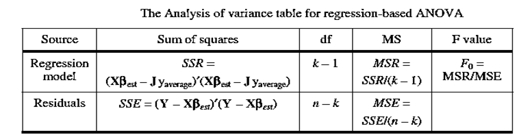
The following are used in the ANOVA method:
1) Ds are the input pattern in the flat file.
2) H and L are the highs and lows respectively of the numbers in each column of the input data, Ds.
3) D is the input data in coded units that range between –1 and 1.
4) X is the design matrix.
5) Xs is the scaled design matrix .
6) n is the number of data points or rows in the flat file.
7) m is the number of factors in the regression model being fitted.
8) k is the number of terms in the regression model being fitted.
9) Y is a vector of response data.
10) yaverageis the average of all n responses in the n dimensional data vector Y.
11) J is an n dimensional vector with all entries equal to 1.
a) It is perhaps most standard to pronounce interactions terms as being significant after the optional scaling in Step 1 has been performed. Further, it is often reasonable to accept evidence levels associated with p-values greater than 0.05.
b) This follows because the decision-maker may be attempting to determine whether any causal relationship might exist rather than proving that one does exist.
c) A modified version of the above method is based on an assumption that the standard deviation of the random error, σ, is believed to be known. This could occur, for example, if an Xbar & R chart was used to study this system output and obtain the process capability,
d) The phrase “random factors” refers to system inputs whose levels are relevant mainly because of their relevance in predicting responses from a large population.
e) For example, the participants are random factors in a drug test because we are not primarily interested in the effects on individuals (the levels) but rather on the effects on a population of people. The formulas in the relevant “ANOVA Table”
f) If random factors are involved, then modified formulas in Montgomery (2000) should be used to develop more believable inferences about the effects of the factors on the larger population.
Example (Single Factor ANOVA Application) Calculate and interpret the results of the ANOVA method followed by multiple t-tests based on the data.
Answer: the pvalue of 0.056 can be considered strong evidence that factor x1 affects the average
response values. Note that since it is not clear whether randomized experimentation has been used, it is not proper to declare that the analysis provides proof.
The “Bonferroni inequality” establishes that if q tests are made each with and α chance of giving a Type I error, the chance of no false alarm on any test is greater than 1 – q × α. Even though additional mathetical results can increase this bounding limit, with even a few tests (e.g., q = 4) approaches based on individual testing offer limited overall coverage unless the values used are very small.
ANOVA followed by t-tests can offer the same guarantee while achieving lower Type II error risks than any procedure based on the Bonferroni inequality.
