SKEDSOFT
Histograms in six-sigma: Components of a Histogram
-
Each vertical bar represents an interval of data or a category of data
-
The x-axis are the measurements
-
The y-axis is the frequency
- All bars are adjacent and will not overlap since they represent a certain interval (group) of measurements at a specified frequency.
- The histogram, when made up of normally distributed data, will form a "bell" curve when a smooth probability density function is produced using kernel smoothing techniques.
-
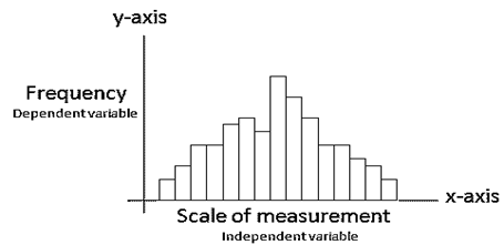
- This line that generalizes the histogram appears to look like a bell.
- Often the more data being analyzed and with more resolution will create more bars since more intervals or categories of data are available to plot. The more measurements and at various frequencies will create more bars and fill up more of the area under the probability density function.
- To assess the data there should be at least 5 bars or intervals and at least 30 data points.
- There are a variety of histograms, for most practical purposes understanding these basic components will be sufficient.
Left-Skewed Distribution (Negatively Skewed):
- These histograms have the curve on the right side or the most common values on the right side of the distribution. The data extends much farther out to the left side.
- These distributions are common where there is an upper specification limit or it is not possible to exceed an upper value, also known as boundary limit.
-
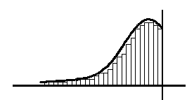
- This may occur if a customer has requested the process run at towards the upper specification limit as opposed to targeting the mean.
- The measure of central location is the median.
- Mean < Median < Mode
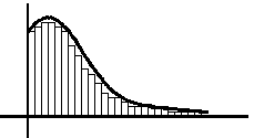
Right Skewed Distribution (Positively Skewed):
- The distribution of the data reaches far out to the right side. This may be caused by a process having a lower boundary. Cost or time plots commonly exhibit this behavior.
- The measure of central location is the median.
- Mode < Median < Mean
- If most common value is 10, the middle most value is 15, and the average of the data set is 20, then the distribution is right skewed.