SKEDSOFT

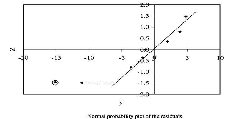
Example(Normal Probability Plotting Residuals) Assume that the residuals are: E_rrorest,1 = –3.6, E_rrorest,2 = –15.1, Errorest,3 = –1.8, E_rrorest,4 = 3.9, E_rrorest,5 = –1.4, E_rrorest,6 = 4.8, and E_rrorest,7 = 2.0. Use normal probability plotting to assess whether any are outliers.

Answer:

 Step 1 gives Z = {–1.47, –0.79, –0.37, 0.00, 0.37, 0.79, 1.47}.

Step 2 gives y_sorted = {–15.1, –3.6, –1.8 –1.4, 2.0, 3.9, 4.8}.

All numbers appear to line up, i.e., seem to come from the samenormal distribution, except for -15.1, which is an outlier. It may be important to investigate the cause of the associated usual response (run 2).

For example, there could be something simple and fixable, such as a data entry error. If found and corrected, a mistake might greatly reduce prediction errors.

        In the context of screening experiments, analysts might normal probability plots the estimated coefficients instead of applying Lenth’s method. The factors judged to be significant (if any) would have coefficients that are outliers.

         In addition to normal probability plotting the residuals, it is common to view plots of the Errorest, i plotted vs yest,i and/or the inputs x_i for each run, i = 1,…,n. For the calculations and associated hypothesis tests to be believable, the E_rrorest ,i values

       should not show an obvious dependence on any other quantities.

       In general, all of these “residual plots” can provide evidence that the functional form needs to be changed and the hypothesis testing results cannot be trusted. Yet, all residual plotting results can also be misleading in cases in which the number of data is comparable to the number of terms in the fitted model.