SKEDSOFT

A few useful random variables:

Recall  that  a  random  variable  X : Ω → R is  called  discrete  if  its  range  (i.e.,  the  set  of  values  that  it  can  take)  is  a  countable  set.  The  PMF  of  X is  a  function  pX : R → [0, 1],  defined  by  pX(x) = P(X = x),  and  completely  determines  the  probability  law  of  X.

The following are some important PMFs.

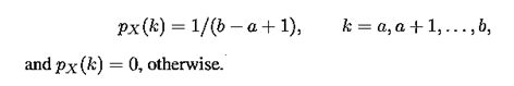
(a)  Discrete  uniform  with  parameters  a and  b,  where  a and  b are  integers  with  a < b.  Here,

(b)  Bernoulli with parameter p, where 0 ≤ p ≤ 1.  Here, PX (0) = p, PX (1) =1 − p.

(c)  Binomial with parameters n and p, where n ∈ N and p ∈ [0, 1].  Here,

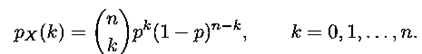
A binomial  random variable  with  parameters n and  p represents  the  number  of  heads  observed  in  n independent  tosses  of  a  coin  if  the  probability  of  heads  at  each  toss  is  p.

(d)  Geometric with parameter p, where 0 < p ≤ 1.  Here,

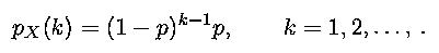
A  geometric  random  variable  with  parameter  p represents  the  number  of  independent  tosses of a  coin  until  heads  are  observed for the  first time, if the  probability  of  heads  at  each  toss  is  p.

(e)  Poisson with parameter λ, where λ > 0.  Here,

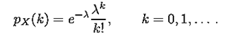
As  will  be  seen  shortly,  a  Poisson  random  variable  can  be  thought  of  as  a  limiting  case  of  a  binomial  random  variable. 

(f)  Power law with parameter α, where α > 0.  Here

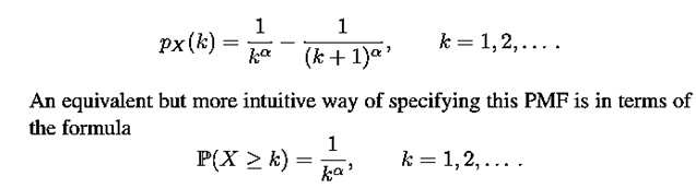
Note  that  when  α is  small,  the  “tail”  P(X ≥ k) of  the  distribution  decays  slowly  (slower  than  an  exponential)  ask increases,  and  in  some  sense  such  a  distribution  has  “heavy”  tails.