SKEDSOFT

Introduction:

Prioritization starts by comparing each row with the columns and asking the question: How important is the row alternative compared to the column alternative? The prioritization matrix, also known as the criteria matrix, is used to compare choices relative to criteria like price, service, ease of use and almost any other factor desired. 

THEORETICAL OUTLINE:

Let i, j entry of the matrix be aij. We then immediately know that the following must hold good of the entries:

aii =1

i.e. the diagonal elements must be equal to unity and the matrix will be reciprocally symmetric.

What we need from this prioritization is a weight describing the relative importance of the four alternatives. Let these weights be w1 to w4 (or in general wn). From this follows that the relationship between the ws and the as must be as follows if the matrix is consistent:                

This leads to the conclusion that                                                                      

And from which, by summation over all alternatives, we find that the following interesting relationship must hold:

The vector of relative weights as the solution to the following matrix equation which is equal to the characteristic equation of the prioritization matrix A:                      Aw=lmaxw

Where lmaxis the largest eigenvalue and w is the corresponding eigen vector.

Inconsistency index will be measured as follows: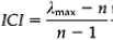  

This number tells us how consistent the decision makers have been when they constructed the prioritization matrix. Saathy has suggested that if the ICI exceeds 0.10 the matrix should be rejected and the process should start over again.

Another method:

The degree of inconsistency is not as easy to calculate if you are not going to use the matrix calculations. The method is as follows:

1. Multiply the columns of the original matrix by the weights of the alternatives;

2. Compute the row sum of the new matrix;

3. Divide the row sums by the weights of the alternatives;

4. Compute the average of the new numbers. This average is an estimate of lmax.

• In step 1 we multiply the columns by the weights of the alternatives. This leads to the following matrix which we may call C:
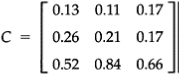
• Now compute the sum of the rows and divide this sum by the weights of the alternatives. This gives.

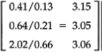
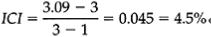
The average of the RHS is now equal to 3.09 from which follows that the ICI is: