SKEDSOFT
CTL syntax: CTL formulas γ are inductively defined as follows:
γ → x a propositional variable
| ¬γ negation of γ
| (γ) parenthesization of γ
| γ1 ∨ γ2 disjunction
| AG γ on all paths, everywhere along each path
| AF γ on all paths, somewhere on each path
| AX γ on all paths, next time on each path
| EG γ on some path, everywhere on that path
| EF γ on some path, somewhere on that path
| EX γ on some path, next time on that path
| A[γ1 U γ2] onallpaths, γ1 until γ2
| E[γ1 U γ2] on some path, γ1 until γ2
| A[γ1 W γ2] onallpaths, γ1 weak-until γ2
| E[γ1 W γ2] on some path, γ1 weak-until γ2
CTL semantics: The semantics of CTL formulas are defined over computation trees. Our approach to defining this semantics recurses over the structure of computation trees. We will also employ fixed-points to capture this semantics precisely. Some of the reasons for taking a different approach6 are the following:
- Some approaches (e.g., [20]) introduce a more general temporal logic (namely CTL∗) and then introduce CTL and LTL as special cases. We wanted to keep our discussions at a more elementary level.
- Our definitions make an explicit connection with the standard fixedpoint semantics of CTL.
- The view of LTL and CTL being Kripke structure classifiers is more readily apparent from our definitions.
Let a computation tree be denoted by τ. Here are the notations we shall use:
- τ = τ ε. We are going to “exponentiate” τ with tree paths as described in Section 15.6.2, with ε denoting the empty sequence.
- The state at τ ε is s(τ ε).
- τ ε has β(τ ε) 1 branches numbered 0 through β(τ ε). In effect, β specifies the arity at every node of the computation tree. Since each Kripke structure has a total state transition relation R, β(τ ) ≥ 0 for any computation tree τ .
- Branch 0 ≤ j ≤ β(τ ε) leads to computation tree τ j (for example, τ 0 is the computation tree rooted at the first child of τ ε, τ 1 is the computation tree rooted at the second child of τ ε, etc).
- Generalizing this notation, for a sequence of natural numbers π, τ π denotes the computation tree arrived at by traversing the branches
- identified in π. We call these the (computation) trees yielded by π (for example, τ 1,0,1,1,2 is a computation tree obtained by traversing the tree path described by 1, 0, 1, 1, 2, starting from τ ε).
- For an arbitrary sequence of natural numbers π, τ π is not defined if any of the natural numbers in the sequence π exceeds the corresponding β value, i.e., the arity of the tree at a certain level. We
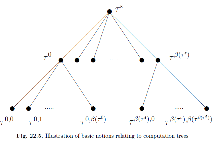
will make sure not to exceed the arity. Hence, s(τ π) is the state that the computation tree τ π is rooted at, and β(τ π) 1 is the number of children it has.
