SKEDSOFT

Introduction to Complexity Theory: There are two kinds of measures with Complexity Theory:

(a) time and

(b) space.

(i) Time Complexity: It is a measure of how long a computation takes to execute. As far as Turing machine is concerned, this could be measured as the number of moves which are required to perform a computation. In the case of a digital computer, this could be measured as the number of machine cycles which are required for the computation.

(ii) Space Complexity: It is a measure of how much storage is required for a computation. In the case of a Turing machine, the obvious measure is the number of tape squares used, for a digital computer, the number of bytes used.

It is to be noted that both these measures functions of a single input parameter, viz., “size of the input”, which is defined in terms of squares or bytes. For any given input size, different inputs require different amounts of space and time. Thus it will be easier to discuss about the “average case” or for the “worst case”. It is usually interesting to look at the worst-case complexity because

(a) It may be difficult to define an “average case”

(b) Usually easier to compute worst-case complexity.

Order Statistic: In Complexity theory, equations are subjected to extreme simplifications. If an algorithm takes exactly 50n3 5n2 - 5n 56 machine cycles, where ‘n’ is the size of the input, then we shall simplify this toO(n3). This is called the “order statistic”. It is customary to

(a) drop all terms except the highest-ordered one

(b) drop the co-efficient of the highest-ordered term.

For very large values of n, the effect of the highest-order term completely swamps the contribution of lower-ordered term. Tweaking the code can improve the coefficients, but the order statisfic is a function of the algorithm itself.

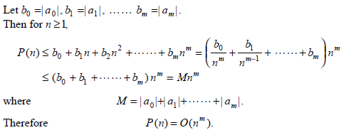
Exam ple 7.1.1: Given 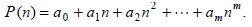Show that

Solution: