SKEDSOFT

Introduction: To determine if there is any “real” difference in the mean error rates of two models, we need to employ a test of statistical significance. In addition, we would like to obtain some confidence limits for our mean error rates so that we can make statements like “any observed mean will not vary by /- two standard errors 95% of the time for future samples” or “one model is better than the other by a margin of error of /- 4%.”

What do we need in order to perform the statistical test? Suppose that for each model, we did 10-fold cross-validation, say, 10 times, each time using a different 10-fold partitioning of the data. Each partitioning is independently drawn. We can average the 10 error rates obtained each for M1 and M2, respectively, to obtain the mean error rate for each model. For a given model, the individual error rates calculated in the cross-validations may be considered as different, independent samples from a probability distribution. In general, they follow a t distribution with k-1 degrees of freedom where, here, k = 10. (This distribution looks very similar to a normal, or Gaussian, distribution even though the functions defining the two are quite different. Both are uni-modal, symmetric, and bell-shaped.) This allows us to do hypothesis testing where the significance test used is the t-test, or Student’s t-test. Our hypothesis is that the two models are the same, or in other words, that the difference in mean error rate between the two is zero. If we can reject this hypothesis (referred to as the null hypothesis), then we can conclude that the difference between the two models is statistically significant, in which case we can select the model with the lower error rate.

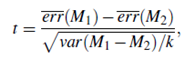
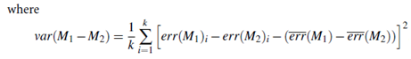
In data mining practice, we may often employ a single test set, that is, the same test set can be used for both M1 and M2. In such cases, we do a pair wise comparison of the two models for each 10-fold cross-validation round. That is, for the ith round of 10-fold cross-validation, the same cross-validation partitioning is used to obtain an error rate for M1 and an error rate for M2. Let err(M1)i (or err(M2)i) be the error rate of model M1 (or M2) on round i. The error rates for M1 are averaged to obtain a mean error rate for M1, denoted err(M1). Similarly, we can obtain err(M2). The variance of the difference between the two models is denoted var(M1-M2). The t-test computes the t-statistic with k-1 degrees of freedom for k samples. In our example we have k = 10 since, here, the k samples are our error rates obtained from ten 10-fold cross-validations for each model. The t-statistic for pair wise comparison is computed as follows:

To determine whether M1 and M2 are significantly different, we compute t and select a significance level, sig. In practice, a significance level of 5% or 1% is typically used. We then consult a table for the t distribution, available in standard textbooks on statistics. This table is usually shown arranged by degrees of freedom as rows and significance levels as columns. Suppose we want to ascertain whether the difference between M1 and M2 is significantly different for 95% of the population, that is, sig = 5% or 0.05. We need to find the t distribution value corresponding to k-1 degrees of freedom (or 9 degrees of freedom for our example) from the table. However, because the t distribution is symmetric, typically only the upper percentage points of the distribution are shown. Therefore, we look up the table value for z = sig=2, which in this case is 0.025, where z is also referred to as a confidence limit. If t > z or t < -z, then our value of t lies in the rejection region, within the tails of the distribution. This means that we can reject the null hypothesis that the means of M1 and M2 are the same and conclude that there is a statistically significant difference between the two models. Otherwise, if we cannot reject the null hypothesis, we then conclude that any difference between M1 and M2 can be attributed to chance.

If two test sets are available instead of a single test set, then a non-paired version of the t-test is used, where the variance between the means of the two models is estimated as

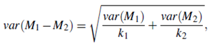
and k1 and k2 are the number of cross-validation samples (in our case, 10-fold cross validation rounds) used for M1 and M2, respectively. When consulting the table of t distribution, the number of degrees of freedom used is taken as the minimum number of degrees of the two models.