SKEDSOFT
Introduction: The degree to which numerical data tend to spread is called the dispersion, or variance of the data. The most common measures of data dispersion are range, the five-number summary (based on quartiles), the inter quartile range, and the standard deviation. Box plots can be plotted based on the five-number summary and are a useful tool for identifying outliers.
Range, Quartiles, Outliers, and Box plots
Let x1;x2; : : : ;xN be a set of observations for some attribute. The range of the set is the difference between the largest (max()) and smallest (min()) values. For the remainder of this section, let’s assume that the data are sorted in increasing numerical order.
The kth percentile of a set of data in numerical order is the value xi having the property that k percent of the data entries lie at or below xi. The median (discussed in the previous subsection) is the 50th percentile.
The most commonly used percentiles other than the median are quartiles. The first quartile, denoted by Q1, is the 25th percentile; the third quartile, denoted by Q3, is the 75th percentile. The quartiles, including the median, give some indication of the center, spread, and shape of a distribution. The distance between the first and third quartiles is a simple measure of spread that gives the range covered by the middle half of the data. This distance is called the inter quartile range (IQR) and is defined as
IQR = Q3 - Q1. (2.5)
Based on reasoning similar to that in our analysis of the median in Section 2.2.1, we can conclude that Q1 and Q3 are holistic measures, as is IQR.
No single numerical measure of spread, such as IQR, is very useful for describing skewed distributions. The spreads of two sides of a skewed distribution are unequal (Figure 2.2). Therefore, it is more informative to also provide the two quartiles Q1 and Q3, along with the median. A common rule of thumb for identifying suspected outliers is to single out values falling at least 1:5IQR above the third quartile or below the first quartile.
BecauseQ1, the median, andQ3 together contain no information about the endpoints (e.g., tails) of the data, a fuller summary of the shape of a distribution can be obtained by providing the lowest and highest data values as well. This is known as the five-number summary. The five-number summary of a distribution consists of the median, the quartilesQ1 andQ3, and the smallest and largest individual observations, written in the order Minimum; Q1; Median; Q3; Maximum:
Box plots are a popular way of visualizing a distribution. A box plot incorporates the five-number summary as follows:
- Typically, the ends of the box are at the quartiles, so that the box length is the inter quartile range, IQR.
- The median is marked by a line within the box.
- Two lines (called whiskers) outside the box extend to the smallest (Minimum) and largest (Maximum) observations.
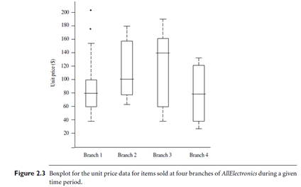 When dealing with a moderate number of observations, it is worthwhile to plot potential outliers individually. To do this in a box plot, the whiskers are extended to the extreme low and high observations only if these values are less than 1:5IQR beyond the quartiles. Otherwise, the whiskers terminate at the most extreme observations occurring within 1:5IQR of the quartiles. The remaining cases are plotted individually. Boxplots can be used in the comparisons of several sets of compatible data. Figure 2.3 shows boxplots for unit price data for items sold at four branches of All Electronics during a given time period. For branch 1, we see that the median price of items sold is $80, Q1 is $60, Q3 is $100. Notice that two outlying observations for this branch were plotted individually, as their values of 175 and 202 are more than 1.5 times the IQR here of 40. The efficient computation of boxplots, or even approximate boxplots (based on approximates of the five-number summary), remains a challenging issue for the mining of large data sets.
Variance and Standard Deviation: The variance of N observations, x1;x2; : : : ;xN, is
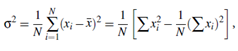
where x is the mean value of the observations, as defined in Equation (2.1). The standard deviation, s, of the observations is the square root of the variance, s2.
The basic properties of the standard deviation, σ, as a measure of spread are
- σ measures spread about the mean and should be used only when the mean is chosen as the measure of center.
- σ =0 only when there is no spread, that is, when all observations have the same value. Otherwise σ > 0.
The variance and standard deviation are algebraic measures because they can be computed from distributive measures. That is, N (which is count() in SQL), åxi (which is the sum() of xi), and åx2 i (which is the sum() of x2 i ) can be computed in any partition.
