SKEDSOFT

ntroduction: The naïve Bayesian classifier, or simple Bayesian classifier, works as follows:

• Let D be a training set of tuples and their associated class labels. As usual, each tuple is represented by an n-dimensional attribute vector, X = (x1, x2, : : : , xn), depicting n measurements made on the tuple from n attributes, respectively, A1, A2, : : : , An.
• Suppose that there are m classes, C1, C2, : : : , Cm. Given a tuple, X, the classifier will predict that X belongs to the class having the highest posterior probability, conditioned on X. That is, the naïve Bayesian classifier predicts that tuple X belongs to the class Ci if and only if

P(Ci|X) > P(Cj|X) for 1 ≤ j ≤ m; j ≠ i:

Thus we maximize P(Ci|X). The class Ci for which P(Ci|X) is maximized is called the maximum posteriori hypothesis. By Bayes’ theorem (Equation (6.10)),

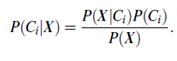
• As P(X) is constant for all classes, only P(X|Ci)P(Ci) need be maximized. If the class prior probabilities are not known, then it is commonly assumed that the classes are equally likely, that is, P(C1) = P(C2) = _ _ _ = P(Cm), and we would therefore maximize P(X|Ci). Otherwise, we maximize P(X|Ci)P(Ci). Note that the class prior probabilities may be estimated by P(Ci)=|C_i,D|/|D|, where |C_i,D| is the number of training tuples of class Ci in D.
• Given data sets with many attributes, it would be extremely computationally expensive to compute P(X|Ci). In order to reduce computation in evaluating P(X|Ci), the naive assumption of class conditional independence is made. This presumes that the values of the attributes are conditionally independent of one another, given the class label of the tuple (i.e., that there are no dependence relationships among the attributes). Thus,

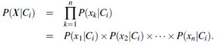
We can easily estimate the probabilities P(x1|Ci), P(x2|Ci), : : : , P(xn|Ci) from the training  tuples. Recall that here xk refers to the value of attribute Ak for tuple X. For each attribute, we look at whether the attribute is categorical or continuous-valued. For instance, to compute P(X|Ci), we consider the following:

(a) If Ak is categorical, then P(xk|Ci) is the number of tuples of class Ci in D having the value xk for Ak, divided by |Ci,D|, the number of tuples of class Ci in D.

(b) If Ak is continuous-valued, then we need to do a bit more work, but the calculation is pretty straightforward. A continuous-valued attribute is typically assumed to have a Gaussian distribution with a mean μ and standard deviation s, defined by

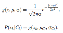
These equations may appear daunting, but hold on We need to compute μCi and σCi , which are the mean (i.e., average) and standard deviation, respectively, of the values of attribute Ak for training tuples of class Ci. We then plug these two quantities into Equation (6.13), together with xk, in order to estimate P(xk|Ci). For example, let X = (35, $40,000), where A1 and A2 are the attributes age and income, respectively. Let the class label attribute be buys computer. The associated class label for X is yes (i.e., buys_computer = yes). Let’s suppose that age has not been discretized and therefore exists as a continuous-valued attribute. Suppose that from the training set, we find that customers in D who buy a computer are 38±12 years of age. In other words, for attribute age and this class, we have μ = 38 years and σ = 12.We can plug these quantities, along with x1 = 35 for our tuple X into Equation (6.13) in order to estimate P(age = 35|buys_computer = yes).

• In order to predict the class label of X, P(X|Ci)P(Ci) is evaluated for each class Ci. The classifier predicts that the class label of tuple X is the class Ci if and only if

P(X|Ci)P(Ci) > P(X|Cj)P(Cj) for 1 ≤ j ≤ m, j ≠ i.  

In other words, the predicted class label is the class Ci for which P(X|Ci)P(Ci) is the maximum.