SKEDSOFT
Introduction: Techniques of numerosity reduction can indeed be applied for reduce the data volume by choosing alternative, ‘smaller’ forms of data representation purpose. These techniques may be parametric or nonparametric. For parametric methods, a model is used to estimate the data, so that typically only the data parameters need to be stored, instead of the actual data. (Outliers may also be stored.) Log-linear models, which estimate discrete multidimensional probability distributions, are an example. Nonparametric methods for storing reduced representations of the data include histograms, clustering, and sampling.
Let’s look at each of the numerosity reduction techniques mentioned above.
Regression and Log-Linear Models: Regression and log-linear models can be used to approximate the given data. In (simple) linear regression, the data are modeled to fit a straight line. For example, a random variable, y (called a response variable), can be modeled as a linear function of another random variable, x (called a predictor variable), with the equation
y = wx b, (2.14)
where the variance of y is assumed to be constant. In the context of data mining, x and y are numerical database attributes. The coefficients, wand b (called regression coefficients), specify the slope of the line and the Y-intercept, respectively. These coefficients can be solved for by the method of least squares, which minimizes the error between the actual line separating the data and the estimate of the line. Multiple linear regressions is an extension of (simple) linear regression, which allows a response variable, y, to be modeled as a linear function of two or more predictor variables.
Log-linear models approximate discrete multidimensional probability distributions. Given a set of tuples in n dimensions (e.g., described by n attributes), we can consider each tuple as a point in an n-dimensional space. Log-linear models can be used to estimate the probability of each point in a multidimensional space for a set of discretized attributes, based on a smaller subset of dimensional combinations. This allows a higher-dimensional data space to be constructed from lower dimensional spaces. Log-linear models are therefore also useful for dimensionality reduction (since the lower-dimensional points together typically occupy less space than the original data points) and data smoothing (since aggregate estimates in the lower-dimensional space are less subject to sampling variations than the estimates in the higher-dimensional space).
Regression and log-linear models can both be used on sparse data, although their application may be limited. While both methods can handle skewed data, regression does exceptionally well. Regression can be computationally intensive when applied to high dimensional data, whereas log-linear models show good scalability for up to 10 or so dimensions.
Histograms: Histograms use binning to approximate data distributions and are a popular form of data reduction. Histograms were introduced in Section 2.2.3. A histogram for an attribute, A, partitions the data distribution of A into disjoint subsets, or buckets. If each bucket represents only a single attribute-value/frequency pair, the buckets are called singleton buckets. Often, buckets instead represent continuous ranges for the given attribute.
Example: Histograms. The following data are a list of prices of commonly sold items at All Electronics (rounded to the nearest dollar). The numbers have been sorted: 1, 1, 5, 5, 5, 5, 5,8, 8, 10, 10, 10, 10, 12, 14, 14, 14, 15, 15, 15, 15, 15, 15, 18, 18, 18, 18, 18, 18, 18, 18, 20,20, 20, 20, 20, 20, 20, 21, 21, 21, 21, 25, 25, 25, 25, 25, 28, 28, 30, 30, 30.
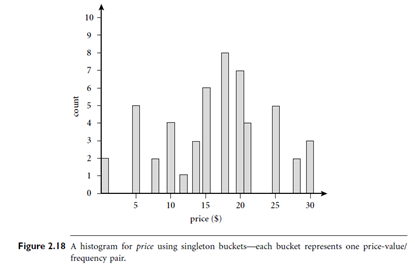
Figure 2.18 shows a histogram for the data using singleton buckets. To further reduce the data, it is common to have each bucket denote a continuous range of values for the given attribute. In Figure 2.19, each bucket represents a different $10 range for price. “How are the buckets determined and the attribute values partitioned?” There are several partitioning rules, including the following:
- Equal-width: In an equal-width histogram, the width of each bucket range is uniform (such as the width of $10 for the buckets in Figure 2.19).
- Equal-frequency (or equidepth):In an equal-frequency histogram, the buckets are created so that, roughly, the frequency of each bucket is constant (that is, each bucket contains roughly the same number of contiguous data samples).
- V-Optimal: If we consider all of the possible histograms for a given number of buckets, the V-Optimal histogram is the one with the least variance. Histogram variance is a weighted sum of the original values that each bucket represents, where bucket weight is equal to the number of values in the bucket.
- Max-Diff:In a Max-Diff histogram, we consider the difference between each pair of adjacent values. A bucket boundary is established between each pair for pairs having the β - 1 largest differences, where β is the user-specified number of buckets.
