SKEDSOFT

Introduction:

In this section, we describe the Star-Cubing algorithm for computing iceberg cubes. Star-Cubing combines the strengths of the other methods we have studied up to this point. It integrates top-down and bottom-up cube computation and explores both multidimensional aggregation (similar to MultiWay) and Apriori-like pruning (similar to BUC). It operates from a data structure called a star-tree, which performs lossless data compression, thereby reducing the computation time and memory requirements.

The Star-Cubing algorithm explores both the bottom-up and top-down computation models as follows: On the global computation order, it uses the bottom-up model. However, it has a sub layer underneath based on the top-down model, which explores the notion of shared dimensions, as we shall see below. This integration allows the algorithm to aggregate onmultiple dimensions while still partitioning parent group-by’s and pruning child group-by’s that do not satisfy the iceberg condition.

Star-Cubing’s approach is illustrated in Figure 4.8 for the computation of a 4-D data cube. If we were to follow only the bottom-up model (similar to Multiway), then the cuboids marked as pruned by Star-Cubing would still be explored. Star-Cubing is able to prune the indicated cuboids because it considers shared dimensions. ACD=A means cuboid ACD has shared dimension A, ABD=AB means cuboid ABD has shared dimension AB, ABC=ABC means cuboid ABC has shared dimension ABC, and so on. This comes from the generalization that all the cuboids in the subtree rooted at ACD include dimension A, all those rooted at ABD include dimensions AB, and all those rooted at ABC include dimensions ABC (even though there is only one such cuboid). We call these common dimensions the shared dimensions of those particular sub trees.

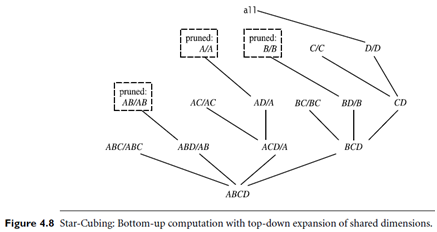
The introduction of shared dimensions facilitates shared computation. Because the shared dimensions are identified early on in the tree expansion, we can avoid re computing them later. For example, cuboid AB extending from ABD in Figure 4.8 would actually be pruned because AB was already computed in ABD=AB. Similarly, cuboid A extending from AD would also be pruned because it was already computed in ACD=A.

Shared dimensions allow us to do A priori-like pruning if the measure of an iceberg cube, such as count, is anti monotonic; that is, if the aggregate value on a shared dimension does not satisfy the iceberg condition, then all of the cells descending from this shared dimension cannot satisfy the iceberg condition either. Such cells and all of their descendants can be pruned, because these descendant cells are, by definition, more specialized (i.e., contain more dimensions) than those in the shared dimension(s). The number of tuples covered by the descendant cells will be less than or equal to the number of tuples covered by the shared dimensions. Therefore, if the aggregate value on a shared dimension fails the iceberg condition, the descendant cells cannot satisfy it either.