SKEDSOFT

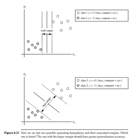
Where W is a weight vector, namely, W = {w1, w2, : : : , wn}; n is the number of attributes; and b is a scalar, often referred to as a bias. To aid in visualization, let’s consider two input attributes, A1 and A2, as in Figure 6.21(b). Training tuples are 2-D, e.g., X = (x1, x2), where x1 and x2 are the values of attributes A1 and A2, respectively, for X. If we think of b as an additional weight, w0, we can rewrite the above separating hyper plane as

w0 w1x1 w2x2 = 0:

Thus, any point that lies above the separating hyper plane satisfies

w0 w1x1 w2x2 > 0

Similarly, any point that lies below the separating hyper plane satisfies

w0 w1x1 w2x2 < 0

The weights can be adjusted so that the hyper planes defining the “sides” of the margin can be written as

H1 : w0 w1x1 w2x2 ≥ 1 for yi = 1, and (6.36)

H2 : w0 w1x1 w2x2 ≤ -1 for yi = -1: (6.37)

That is, any tuple that falls on or above H1 belongs to class 1, and any tuple that falls on or below H2 belongs to class ---1. Combining the two inequalities of Equations (6.36) and (6.37), we get

yi(w0 w1x1 w2x2) ≥ 1, ∀i. (6.38)

Any training tuples that fall on hyper planes H1 or H2 (i.e., the “sides” defining the margin) satisfy Equation (6.38) and are called support vectors. That is, they are equally close to the (separating) MMH. In Figure 6.22, the support vectors are shown encircled with a thicker border. Essentially, the support vectors are the most difficult tuples to classify and give the most information regarding classification. From the above, we can obtain a formulae for the size of the maximal margin. The distance from the separating hyper plane to any point on H1 is 1 /||W||, where ||W|| is the Euclidean norm of W,that is p

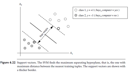
√(WW). By definition, this is equal to the distance from any point on H2 to the separating hyper plane. Therefore, the maximal margin is 2 /||W||.

“So, how does an SVM find the MMH and the support vectors?”Using some “fancy math tricks,” we can rewrite Equation (6.38) so that it becomes what is known as a constrained (convex) quadratic optimization problem. Such fancy math tricks are beyond the scope of this book. Advanced readers may be interested to note that the tricks involve rewriting Equation using a Lagrangian formulation and then solving for the solution using Karush-Kuhn-Tucker (KKT) conditions. Details can be found in references at the end of this chapter. If the data are small (say, less than 2,000 training tuples), any optimization software package for solving constrained convex quadratic problems can then be used to find the support vectors and MMH. For larger data, special and more efficient algorithms for training SVMs can be used instead, the details of which exceed the scope of this book. Once we’ve found the support vectors and MMH (note that the support vectors define the MMH!), we have a trained support vector machine. The MMH is a linear class boundary, and so the corresponding SVM can be used to classify linearly separable data. We refer to such a trained SVM as a linear SVM.