SKEDSOFT

Greedy versus dynamic programming

Because the optimal-substructure property is exploited by both the greedy and dynamic-programming strategies, one might be tempted to generate a dynamic-programming solution to a problem when a greedy solution suffices, or one might mistakenly think that a greedy solution works when in fact a dynamic-programming solution is required. To illustrate the subtleties between the two techniques, let us investigate two variants of a classical optimization problem.

The 0-1 knapsack problem is posed as follows. A thief robbing a store finds n items; the ith item is worth v_i dollars and weighs w_i pounds, where v_i and w_i are integers. He wants to take as valuable a load as possible, but he can carry at most W pounds in his knapsack for some integer W. Which items should he take? (This is called the 0-1 knapsack problem because each item must either be taken or left behind; the thief cannot take a fractional amount of an item or take an item more than once.)

In the fractional knapsack problem, the setup is the same, but the thief can take fractions of items, rather than having to make a binary (0-1) choice for each item. You can think of an item in the 0-1 knapsack problem as being like a gold ingot, while an item in the fractional knapsack problem is more like gold dust.

Both knapsack problems exhibit the optimal-substructure property. For the 0-1 problem, consider the most valuable load that weighs at most W pounds. If we remove item j from this load, the remaining load must be the most valuable load weighing at most W - w_j that the thief can take from the n - 1 original items excluding j. For the comparable fractional problem, consider that if we remove a weight w of one item j from the optimal load, the remaining load must be the most valuable load weighing at most W - w that the thief can take from the n - 1 original items plus w_j - w pounds of item j.

Although the problems are similar, the fractional knapsack problem is solvable by a greedy strategy, whereas the 0-1 problem is not. To solve the fractional problem, we first compute the value per pound v_i/w_i for each item. Obeying a greedy strategy, the thief begins by taking as much as possible of the item with the greatest value per pound. If the supply of that item is exhausted and he can still carry more, he takes as much as possible of the item with the next greatest value per pound, and so forth until he can't carry any more. Thus, by sorting the items by value per pound, the greedy algorithm runs in O(n lg n) time.

To see that this greedy strategy does not work for the 0-1 knapsack problem, consider the problem instance illustrated in Figure 16.2(a). There are 3 items, and the knapsack can hold 50 pounds. Item 1 weighs 10 pounds and is worth 60 dollars. Item 2 weighs 20 pounds and is worth 100 dollars. Item 3 weighs 30 pounds and is worth 120 dollars. Thus, the value per pound of item 1 is 6 dollars per pound, which is greater than the value per pound of either item 2 (5 dollars per pound) or item 3 (4 dollars per pound). The greedy strategy, therefore, would take item 1 first. As can be seen from the case analysis in Figure 16.2(b), however, the optimal solution takes items 2 and 3, leaving 1 behind. The two possible solutions that involve item 1 are both suboptimal.

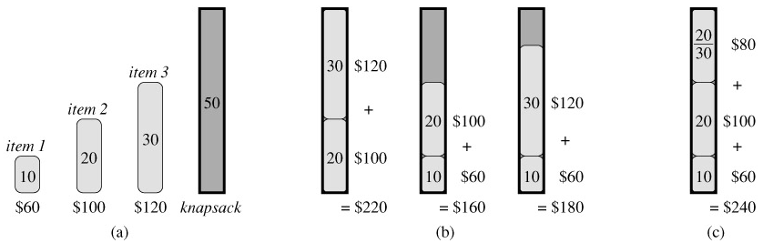
For the comparable fractional problem, however, the greedy strategy, which takes item 1 first, does yield an optimal solution, as shown in Figure 16.2(c). Taking item 1 doesn't work in the 0-1 problem because the thief is unable to fill his knapsack to capacity, and the empty space lowers the effective value per pound of his load. In the 0-1 problem, when we consider an item for inclusion in the knapsack, we must compare the solution to the subproblem in which the item is included with the solution to the subproblem in which the item is excluded before we can make the choice. The problem formulated in this way gives rise to many over-lapping subproblems-a hallmark of dynamic programming, and indeed, dynamic programming can be used to solve the 0-1 problem.