SKEDSOFT

We next show that at most 8 points of P can reside within this δ × 2δ rectangle. Consider the δ × δ square forming the left half of this rectangle. Since all points within P_L are at least δ units apart, at most 4 points can reside within this square; Figure 33.11(b) shows how. Similarly, at most 4 points in P_R can reside within the δ × δ square forming the right half of the rectangle. Thus, at most 8 points of P can reside within the δ × 2δ rectangle. (Note that since points on line l may be in either P_L or P_R, there may be up to 4 points on l. This limit is achieved if there are two pairs of coincident points such that each pair consists of one point from P_L and one point from P_R, one pair is at the intersection of l and the top of the rectangle, and the other pair is where l intersects the bottom of the rectangle.)

Having shown that at most 8 points of P can reside within the rectangle, it is easy to see that we need only check the 7 points following each point in the array Y′.Still assuming that the closest pair is p_L and p_R, let us assume without loss of generality that p_L precedes p_R in array Y′. Then, even if p_L occurs as early as possible in Y′ and p_R occurs as late as possible, p_R is in one of the 7 positions following p_L . Thus, we have shown the correctness of the closest-pair algorithm.

Implementation and running time: As we have noted, our goal is to have the recurrence for the running time be T(n) = 2T(n/2) O(n), where T(n) is the running time for a set of n points. The main difficulty is in ensuring that the arrays X_L, X_R, Y_L, and Y_R, which are passed to recursive calls, are sorted by the proper coordinate and also that the array Y′ is sorted by y-coordinate. (Note that if the array X that is received by a recursive call is already sorted, then the division of set P into P_L and P_R is easily accomplished in linear time.)

The key observation is that in each call, we wish to form a sorted subset of a sorted array. For example, a particular invocation is given the subset P and the array Y , sorted by y-coordinate. Having partitioned P into P_L and P_R, it needs to form the arrays Y_L and Y_R, which are sorted by y-coordinate. Moreover, these arrays must be formed in linear time. The method can be viewed as the opposite of the MERGE procedure from merge sort in The divide-and-conquer approach: we are splitting a sorted array into two sorted arrays. The following pseudocode gives the idea.

	1  length[YL] ← length[YR] ← 0
2  for i ← 1 to length[Y]
3       do if Y[i] ∈ PL
4             then length[YL] ← length[YL]   1
5                  YL[length[YL]] ← Y[i]
6             else length[YR] ← length[YR]   1
7                  YR[length[YR]] ← Y[i]

We simply examine the points in array Y in order. If a point Y[i] is in P_L, we append it to the end of array Y_L; otherwise, we append it to the end of array Y_R. Similar pseudocode works for forming arrays X_L, X_R, and Y′.

The only remaining question is how to get the points sorted in the first place. We do this by simply presorting them; that is, we sort them once and for all before the first recursive call. These sorted arrays are passed into the first recursive call, and from there they are whittled down through the recursive calls as necessary. The presorting adds an additional O(n lg n) to the running time, but now each step of the recursion takes linear time exclusive of the recursive calls. Thus, if we let T(n) be the running time of each recursive step and T′(n) be the running time of the entire algorithm, we get T′(n) = T (n) O(n lg n) and

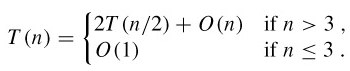
Thus, T(n) = O(n lg n) and T′(n) = O(n lg n).