SKEDSOFT

Reductions: The above notion of showing that one problem is no harder or no easier than another applies even when both problems are decision problems. We take advantage of this idea in almost every NP-completeness proof, as follows. Let us consider a decision problem, say A, which we would like to solve in polynomial time. We call the input to a particular problem an instance of that problem; for example, in PATH, an instance would be a particular graph G, particular vertices u and v of G, and a particular integer k. Now suppose that there is a different decision problem, say B, that we already know how to solve in polynomial time. Finally, suppose that we have a procedure that transforms any instance α of A into some instance β of B with the following characteristics:

1. The transformation takes polynomial time.

2. The answers are the same. That is, the answer for α is "yes" if and only if the answer for β is also "yes."

We call such a procedure a polynomial-time reduction algorithm and, as Figure 34.1 shows, it provides us a way to solve problem A in polynomial time:

1. Given an instance α of problem A, use a polynomial-time reduction algorithm to transform it to an instance β of problem B.

2. Run the polynomial-time decision algorithm for B on the instance β.

3. Use the answer for β as the answer for α.

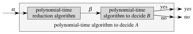
As long as each of these steps takes polynomial time, all three together do also, and so we have a way to decide on α in polynomial time. In other words, by "reducing" solving problem A to solving problem B, we use the "easiness" of B to prove the "easiness" of A.

Recalling that NP-completeness is about showing how hard a problem is rather than how easy it is, we use polynomial-time reductions in the opposite way to show that a problem is NP-complete. Let us take the idea a step further, and show how we could use polynomial-time reductions to show that no polynomial-time algorithm can exist for a particular problem B. Suppose we have a decision problem A for which we already know that no polynomial-time algorithm can exist. (Let us not concern ourselves for now with how to find such a problem A.) Suppose further that we have a polynomial-time reduction transforming instances of A to instances of B. Now we can use a simple proof by contradiction to show that no polynomial-time algorithm can exist for B. Suppose otherwise, i.e., suppose that B has a polynomial-time algorithm. Then, using the method shown in Figure 34.1, we would have a way to solve problem A in polynomial time, which contradicts our assumption that there is no polynomial-time algorithm for A.

For NP-completeness, we cannot assume that there is absolutely no polynomial-time algorithm for problem A. The proof methodology is similar, however, in that we prove that problem B is NP-complete on the assumption that problem A is also NP-complete.