SKEDSOFT
NP-completeness and reducibility: Perhaps the most compelling reason why theoretical computer scientists believe that P ≠ NP is the existence of the class of "NP-complete" problems. This class has the surprising property that if any NP-complete problem can be solved in polynomial time, then every problem in NP has a polynomial-time solution, that is, P = NP. Despite years of study, though, no polynomial-time algorithm has ever been discovered for any NP-complete problem.
The language HAM-CYCLE is one NP-complete problem. If we could decide HAM-CYCLE in polynomial time, then we could solve every problem in NP in polynomial time. In fact, if NP - P should turn out to be nonempty, we could say with certainty that HAM-CYCLE ∈ NP - P.
The NP-complete languages are, in a sense, the "hardest" languages in NP. In this section, we shall show how to compare the relative "hardness" of languages using a precise notion called "polynomial-time reducibility." Then we formally define the NP-complete languages, and we finish by sketching a proof that one such language, called CIRCUIT-SAT, is NP-complete. In NP-completeness proofs and NP-complete problems, we shall use the notion of reducibility to show that many other problems are NP-complete.
Reducibility: Intuitively, a problem Q can be reduced to another problem Q′ if any instance of Q can be "easily rephrased" as an instance of Q′, the solution to which provides a solution to the instance of Q. For example, the problem of solving linear equations in an indeterminate x reduces to the problem of solving quadratic equations. Given an instance ax b = 0, we transform it to 0x2 ax b = 0, whose solution provides a solution to ax b = 0. Thus, if a problem Q reduces to another problem Q′, then Q is, in a sense, "no harder to solve" than Q′.
Returning to our formal-language framework for decision problems, we say that a language L1 is polynomial-time reducible to a language L2, written L1 ≤P L2, if there exists a polynomial-time computable function f : {0, 1}* → {0,1}* such that for all x {0, 1}*,
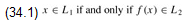
We call the function f the reduction function, and a polynomial-time algorithm F that computes f is called a reduction algorithm.
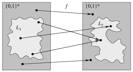
Figure 34.4 illustrates the idea of a polynomial-time reduction from a language L1 to another language L2. Each language is a subset of {0, 1}*. The reduction function f provides a polynomial-time mapping such that if x ∈ L1, then f(x) ∈ L2. Moreover, if x ∉ L1, then f (x) ∉ L2. Thus, the reduction function maps any instance x of the decision problem represented by the language L1 to an instance f (x) of the problem represented by L2. Providing an answer to whether f(x) ∈ L2 directly provides the answer to whether x ∈ L1
Polynomial-time reductions give us a powerful tool for proving that various languages belong to P.
NP-completeness: Polynomial-time reductions provide a formal means for showing that one problem is at least as hard as another, to within a polynomial-time factor. That is, if L1 ≤P L2, then L1 is not more than a polynomial factor harder than L2, which is why the "less than or equal to" notation for reduction is mnemonic. We can now define the set of NP-complete languages, which are the hardest problems in NP.
A language L ⊆ {0, 1}* is NP-complete if
-
L ∈ NP, and
-
L′ ≤P L for every L∈ NP.
If a language L satisfies property 2, but not necessarily property 1, we say that L is NP-hard. We also define NPC to be the class of NP-complete languages.
As the following theorem shows, NP-completeness is at the crux of deciding whether P is in fact equal to NP.
Proof Suppose that L ∈ P and also that L ∈ NPC. For any L′ ∈ NP, we have L′ ≤P L by property 2 of the definition of NP-completeness. we also have that L′ ∈ P, which proves the first statement of the theorem.
To prove the second statement, note that it is the contrapositive of the first statement.
It is for this reason that research into the P ≠ NP question centers around the NP-complete problems. Most theoretical computer scientists believe that P ≠ NP, which leads to the relationships among P, NP, and NPC shown in Figure 34.6. But, for all we know, someone may come up with a polynomial-time algorithm for an NP-complete problem, thus proving that P = NP. Nevertheless, since no polynomial-time algorithm for any NP-complete problem has yet been discovered, a proof that a problem is NP-complete provides excellent evidence for its intractability.
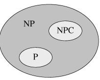
Figure 34.6: How most theoretical computer scientists view the relationships among P, NP, and NPC. Both P and NPC are wholly contained within NP, and P ∩ NPC = Ø.
